

On this page
Axes, scales and text
Scales map your values into physical plot coordinates. Axes use those same
scales, then reserve space for tick labels and axis names. Cartesian y increases
upward. Plot dimensions and text sizes are in millimetres; strings such as
'8pt' work for physical lengths too.
Choose a linear scale for additive differences, a log scale for multiplicative
changes across orders of magnitude, and a categorical scale when order is
nominal. A scale changes visual spacing; it does not transform the source data.
Choose coordinates
| Data | Scale |
|---|---|
| Numeric values | x=(0, 10) or i.linear((0, 10)) |
| Positive values spanning orders of magnitude | i.log((1, 1000)) |
| Values on either side of zero with a compressed outer range | i.symlog((-100, 100)) |
| Named categories | x=['Control', 'Treatment'] or a shared category scale |
| Dates and times | i.dates((start, end)) |
| A deliberate omission in a numeric range | i.broken(...); disclose the break in the caption |
Numeric domain limits do not clip marks automatically. Set clip=True on the
plot when marks should stop at its boundary. A categorical y scale starts at the
bottom; reverse the category order for top-to-bottom reading.
Check that the domain includes the comparisons you intend to make. A truncated
numeric axis can be useful for a measured detail, but disclose it and avoid
reading bar lengths as ratios when zero is outside the view.
Dot plot with named rows
A labelled dot-and-whisker plot puts names down the y axis and values across x.
Give the full model a band of the names as its y scale: each name gets one row,
and the names are the tick labels, so no formatter maps positions back to names.
The first category sits at the bottom, so reverse the list to read top-down.
import inklet as i

countries = ['Chile', 'Peru', 'Brazil', 'Mexico']
ratio = [1.2, 0.8, 2.1, 1.6]
low = [0.9, 0.5, 1.7, 1.1]
high = [1.5, 1.2, 2.6, 2.0]

p = i.plot_spec(60, 40, x=(0, 3), y=i.band(countries[::-1]))
rows = list(zip(ratio, countries))
p.errorbars(rows, xerr=[(r - lo, hi - r) for r, lo, hi in zip(ratio, low, high)], cap=0)
p.scatter(rows, name='Ratio', size=2.2)
p.axes(x='Ratio (95% CI)')
For a table of estimates with intervals, i.quick.forest(df, label=..., estimate=...,
lower=..., upper=...) lays out the same rows with the numbers beside them. It
draws square markers, sized by weight= when you give one.
Tick labels
count=5 requests approximately five intervals. ticks=[...] specifies values
explicitly. format accepts a callable, a format string such as '{:.1f}', or a
suffix. si=True formats a shared SI prefix. Date axes write the year on their
first tick and wherever it changes, so they need no offset; offset="text"
adds a note past the last tick, and offset=False adds nothing.
Continuous scales thin labels when needed. Category labels remain visible by
default. Pass thin=False to keep every requested tick, or thin=True to allow
thinning. Explicit ticks= that thinning drops are listed by figure.report()
as TICKS_DROPPED; no Python warning is issued. rotate=45 rotates tick
labels anticlockwise; it does not rotate the axis name. labels=False keeps
rules and ticks on an interior shared axis. If labels still collide, widen the panel, reduce the requested tick count, or
use a shorter formatter. Inklet does not automatically shrink the text.
Measured typography
Inklet measures font overrides before thinning and layout.
font_size sets the base size for text and spacing; tick_font_size and
label_font_size control those roles independently. font_family, font_weight
and font_style select the measured face. Explicit prebuilt axis-label diagrams
keep their authored size.
import inklet as i

p = i.plot_spec(x=(1000, 9000), y=(0, 1), height=40)
p.line([(1000, .1), (4000, .6), (9000, .85)], stroke='#176b9b')
x_ticks = {'count': 8, 'font_size': '9pt', 'font_weight': 'bold'}
p.grid(y=False, x_options=x_ticks)
p.axis('bottom', label='Frequency / Hz', label_font_size='10pt', **x_ticks)
p.axis('left', label='Response', tick_font_size='8pt', label_font_size='9pt')
doc = i.document(width=110)
doc.add('response', p)
doc.save('axes.svg', 'axes.pdf')
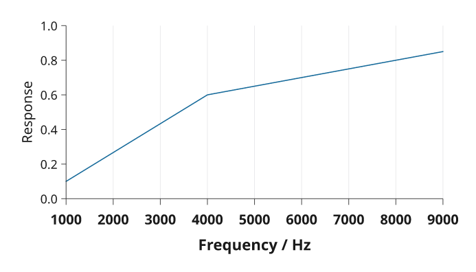
Rendered from the code above.
Pass the same tick-selection options to grid(x_options=..., y_options=...)
and the corresponding axis to keep gridlines aligned with the ticks that remain
visible. These dictionaries accept tick_values() options; axis-only settings
such as label or tick_size do not belong in them. Grid styling, for example
stroke, remains a separate keyword.
Colorbars accept the same font sizes and face overrides. A large tick label can cause fewer values to be shown; use a longer bar or explicit ticks if needed. Text is never reduced to make the labels fit.
More than one scale
Use shared scales for panels that should be compared directly. A secondary axis
from twin_y() or twin_x() has an independent scale; colour it to identify its
series and label its units. See plotting for a complete example,
layout for shared axes, and advanced controls
for categorical groups and external insets.
Use a secondary axis only when the two variables have a clear correspondence;
otherwise separate panels prevent an apparent relationship created by arbitrary
rescaling.