

On this page
Historical material
This page preserves an earlier release or study. See the current guide for supported behavior.
Offline browser rendering
For ordinary native figures, the new compiled-scene viewer adds a WebGL2 circle path with Canvas fallback. This guide covers the existing keyed-row interaction runtime.
Available in 4.0.0.dev1. See the development-preview installation guide.
For the newer mixed line, bar and scatter workflow, see Linked plots. This page retains the original scatter study.
This development preview adds direct picking, linked selection, filtering and
page navigation to measured scatter plots. It lives in
inklet.experimental.browser in the development checkout and is not included
in PyPI 3.1.0. The API and state schema may change.
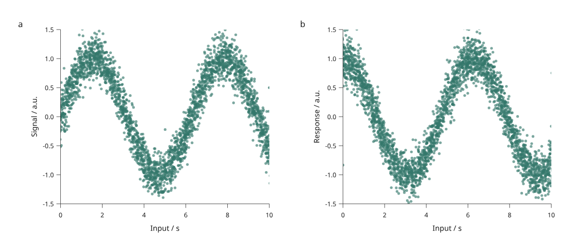
Open the interactive example · Python source · Backend decision and measurements
The example contains 3,000 original simulated observations. Each row connects a signal point and a response point. One missing signal coordinate is omitted in that panel. Points at and just outside the domain edges exercise clipping. Captions and controls remain outside the scientific artwork.
Try the complete workflow
- Open the example and click a point. Both panels select the same row. Shift-click adds or removes rows; table buttons provide keyboard selection.
- Enter part of a row ID to filter observations. A hidden selection remains selected and is counted in the status text.
- Drag to pan, or focus the plot and use arrow keys. Use Zoom in, Zoom
out and Fit page, or the
+,-and0keys. - Choose Save view, change the selection, then Open saved view to restore the filter, selection and viewport.
- Choose Download vector SVG. All three display backends export clipped vector points with the same measured axes and outlined text.
Page zoom enlarges or moves the existing drawing. It does not change data domains, generate ticks or recompile the layout. Hover values and noninteger table numbers use six significant digits for display; integer table values and embedded source values retain their precision. The HTML includes its data, runtime and glyph outlines and works without a server, remote fonts or network requests.
Build and reconstruct in Python
From a development checkout:
python examples/v4/browser_scatter.py --count 3000 --output out/v4-browser
# Open index.html, select/filter/zoom, and download view.json.
python examples/v4/browser_scatter.py --count 3000 --state /path/to/view.json --output out/v4-restored
The second command reconstructs figure.svg and copies the validated state to
view.json. Its HTML now opens with that same saved view already applied. Use the same row count, source data and scene layout.
Changed revisions are rejected rather than silently applied to different rows.
A minimal scene can be built without the optional raster or numerical packages:
from inklet.selection import KeyedTable
from inklet.experimental.browser import BrowserScatter, ScatterView

table = KeyedTable("measurements", {
    "id": ["sample-a", "sample-b", "sample-c"],
    "time": [0, 1, 2],
    "value": [1, 3, 2],
})
scene = BrowserScatter(table, [
    ScatterView("response", "time", "value", (0, 2), (0, 4),
                x_label="Time / s", y_label="Response / a.u.")
])
from pathlib import Path
Path("figure.html").write_text(scene.to_html(backend="svg"))
Path("figure.svg").write_text(scene.to_svg())
BrowserScatter supports one to four views with explicit finite linear domains,
circular markers and numeric or null coordinate columns. Reversed domains work.
The input is an immutable keyed table. Browser visibility accepts arbitrary ID
subsets; the example supplies a simple ID text filter. It does not offer data
upload, brushing, domain rescaling or arbitrary plot types.
Display backends
| Backend | Point layer | Axes and text | Use in this preview |
|---|---|---|---|
| SVG | Vector SVG circles | Outlined SVG | API default; small figures and inspection |
| Canvas | Canvas 2D circles | Rasterized measured SVG frame | Comparison backend; text softens under zoom |
| Hybrid | Canvas 2D circles | Outlined SVG, with vector selection rings | Explicit default in the 3,000-row example |
A local two-panel study measured median redraw submission times of 22.0 ms for SVG and 8.2 ms for hybrid at 3,000 rows; at 20,000 rows, 156.1 ms and 47.9 ms. These are CPU submission timings on one browser/environment, not complete interaction latency or universal crossover thresholds. See the methods, raw records and limitations.
Fidelity and state checks
Picking uses a spatial index in physical page coordinates and respects each panel's clip rectangle and visible IDs. It chooses the nearest eligible center; exact-distance ties follow later source paint order. Pointer handling adds a four-CSS-pixel tolerance. A center outside the domain can contribute a clipped edge, but clicks outside the plot rectangle never select it.
Saved views include a schema version, scene digest, keyed-table revision, selected/visible IDs and viewport. Invalid revisions, unknown or duplicate IDs, and invalid viewports fail before changing the selected/visible state. Null visibility means all rows; an empty list means no rows. Page zoom is bounded from 0.01× to 100×. An old scene cannot be rebased implicitly.
The browser tests cover device pixel ratios 1 and 2, clipping, hidden selections, coordinate conversion, invalid loads and multiple renderer instances. The indexed picker matched an independent exhaustive query for all 1,800 sampled queries in the backend study. Browser SVG downloads and Python reconstruction produced identical pixels at 150 dpi for the checked fit-page and zoomed/panned states. Their XML serialization differs. These bounded checks do not establish pixel identity between canvas and SVG; their edge antialiasing differs.