Microscopy channels and label contours¶

Introduced in Inklet 3.1, Channel, Composite and LabelContour are available from inklet.volume. Install the volume extra from PyPI with pip install "inklet[volume,render]>=4.3". The inklet.experimental import paths used before 4.3 still work and return the same objects.

Channels control display color and windowing without changing sampled intensity values. Contours trace the exact edges of a sampled integer label mask and keep source-coverage limits separate from observed boundaries.

A complete example¶

This example uses simulated signals and labels. Real multichannel data are shown in the fluorescence example.

import numpy as np
import inklet as i
from inklet.volume import Volume, Plane, Channel, Composite

z, y, x = np.indices((9, 41, 51))
radius = (x-25)**2 + (y-20)**2
signal = Volume(100*np.exp(-radius/90), (.5, .2, .2), 'um', source_id='simulated signal')
ring = Volume(80*np.exp(-((np.sqrt(radius)-11)/2)**2),
              (.5, .2, .2), 'um', source_id='simulated ring')
labels = Volume((radius < 80).astype('uint64')*157,
                (.5, .2, .2), 'um', source_id='simulated labels')
plane = Plane((5, 4, 2), (1, 0, 0), (0, 1, 0), (41, 51), (.2, .2), 'um')

channels = (
    Channel('Signal', signal.reslice(plane, kind='intensity'), '#ff00ff', (0, 100)),
    Channel('Ring', ring.reslice(plane, kind='intensity'), '#00ffff', (0, 80)),
)
composite = Composite(channels, coverage='intersection')
contour = labels.reslice(plane, kind='labels').contours(157)
image = i.overlay([
    composite.diagram(width=100),
    contour.diagram(width=100, stroke='#ffd166', coverage='dash'),
], align='origin')

doc = i.document(width=120, columns=1, margin=8)
doc.add('image', image)
doc.add('scale', plane.scalebar(2, width=100))
doc.add('legend', composite.legend())
figure = doc.compile()

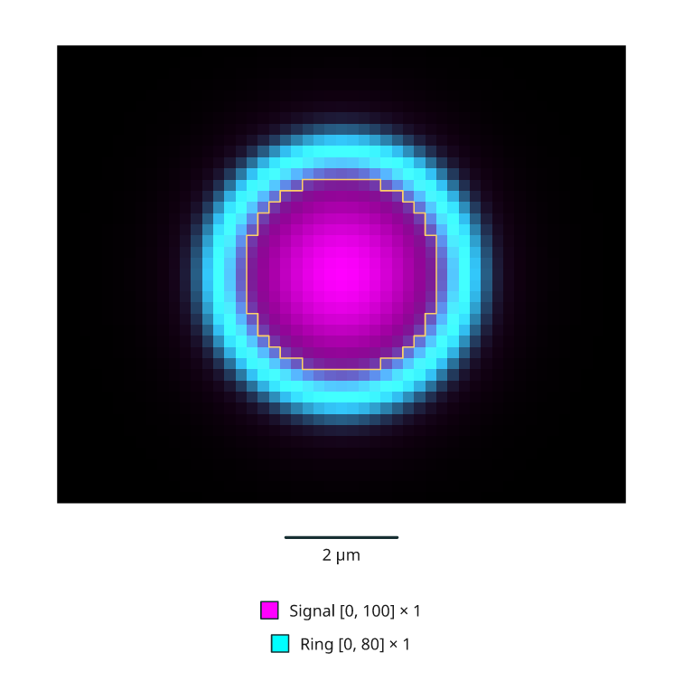
Rendered from the code above.

Use per-label intensity measurements to quantify the unwindowed channel values underlying these images. TIFF import provides named, calibrated scalar volumes for local acquisitions.

Channel display contracts¶

Channel(name, sampled, color, window, weight=1) accepts an intensity SampledSection or a SlabProjection. It rejects label sections. Colors are explicit CSS display colors, not automatically inferred emission wavelengths. Each channel has a finite increasing display window and a weight in (0, 1]. Omit a channel to disable it. Channel names must be unique within a composite.

Composite(channels, coverage=...) requires an explicit coverage choice:

• intersection: a pixel is visible only where every channel has data.
• union: a pixel is visible where any channel has data; an unavailable channel adds no display signal. Missing channels can therefore change the apparent color. The coverage report and channel_counts retain that fact.

All channels must use exactly the same plane geometry. Slab channels must also share thickness and depth sampling; a centre section cannot silently be merged with a thick slab. Sources may have different native grids, but they must be resampled onto the same physical plane or slab. This validates supplied geometry; it does not perform or verify biological image registration.

For each valid channel, display intensity is clip((value - low)/(high - low), 0, 1) * weight. Multiply it by the channel's RGB color and add the channels. The final RGB sum is clipped to [0, 1], then rounded to 8-bit values. This is additive display RGB, without a gamma transform or a physical light model. The ImageJ channel implementation also describes additive RGB channel display. Raw sampled arrays remain unchanged.

composite.rgba, valid and channel_counts are immutable snapshots. composite.report() records each source, window, weight, below/above-window counts, coverage policy and the number of displayed pixels with RGB clipping. composite.legend() creates vector keys with the same names and display ranges. There is no automatic contrast adjustment or inferred colocalization result.

A slab pixel is available when at least one depth sample contributes to that channel. Composite intersection means all channels are available at an output pixel; it does not guarantee identical contributing depths. Inspect each channel's slab counts when coverage differs. Different reductions, if supplied, remain recorded separately in channel provenance. Partial-depth pixels retain the projection API's full display opacity.

Label contour contracts¶

section.contours(label) requires a label SampledSection and a nonnegative integer ID, including exact uint64 values. Background ID 0 is allowed, and an absent ID produces empty boundary sets. Labels retain their identity; this API does not segment an intensity image or infer objects.

The result has two immutable tuples of edge pairs in fractional output YX pixel coordinates:

• observed_yx: an edge separates the selected label from a different label, with both samples valid.
• coverage_yx: an edge separates a selected valid pixel from an invalid neighbour or the image extent. It does not establish an object boundary.

Edges follow pixel sides at half-indices. Holes and disconnected components remain present. Collinear segments are merged, with no smoothing, diagonal interpolation or invented closure across missing data. These are boundary segments, not oriented polygon rings or a connected-component classification. Adjacent label IDs share an edge; overlaying both contours can draw that edge twice, so use explicit colors and ordering.

contour.diagram(width=..., stroke=..., coverage='omit') draws vector paths aligned with the section image. Coverage limits are omitted by default; use 'dash' to distinguish them, or 'show' to draw them solid deliberately. world_segments() returns observed edge pairs in calibrated XYZ for 3D paths; include_coverage=True explicitly includes coverage edges.

contour.report() records label ID, sampled area, observed and coverage lengths, source identity and plane calibration. Length is the pixel-edge estimator on this output grid, not a smooth biological perimeter. Section area is the existing sampled pixel-count estimate, not volume. Resampling resolution can change both. Vector output preserves these sampled boundaries at any page size; it does not increase the measurement resolution.