

On this page
Clipping curves and painted content
Use clip() when the remaining geometry should determine layout. Use
window() when a fixed region should crop all painted content, including
images, glyphs, markers, stroke widths and rounded corners. Both take a Rect
or a convex polygon in the coordinate frame of the supplied drawings.
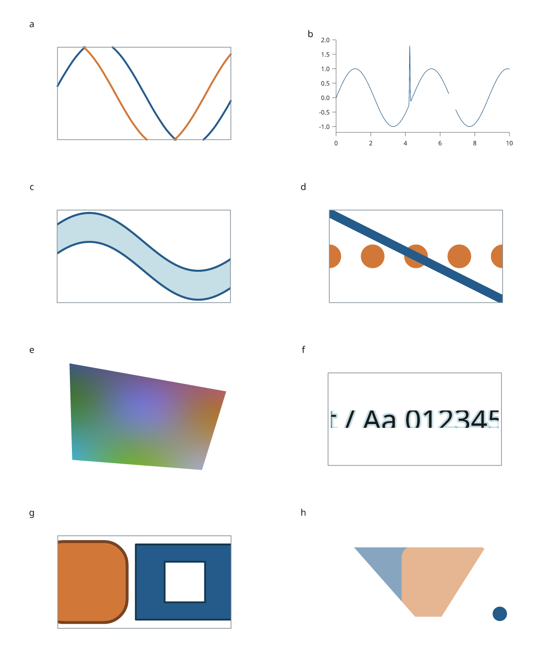
The complete recipe builds all eight panels. The separate caption describes the simulated data, explicit gap and rendering checks. There are no titles or captions inside the figure. Panel f deliberately cuts through glyphs to test paint clipping; it is not a recommended label layout.
Geometric clipping
import inklet as i

line = i.curve([(-20, 0), (-7, 14), (7, -14), (20, 0)],
               stroke="#245b8a", stroke_width=0.5)
cut = i.clip(line, i.Rect(-12, -8, 12, 8))
i.save_svg(cut, "curve.svg", margin=2)
Open cubic paths retain exact subdivided Bézier controls. Intersections with each boundary are isolated between derivative roots and refined by bisection. Repeated exits and reentries remain separate runs; no line joins a removed interval. Rotation, reflection and nonuniform scaling are included when finding intersections in the region's frame.
The accompanying measurement polyline is adaptively flattened to a control polygon/chord tolerance of 0.0001 mm in the clip frame, with a maximum of 65,536 segments per retained cubic. This is not a relative tolerance in data units. Later scaling also scales that measurement tolerance. SVG and PDF use the retained controls, rather than this polyline.
Filled paths are clipped as polygon rings. Their measurement samples determine
the cut, and geometric rectangle cuts do not preserve rounded corners. Use
window() for faithful painted clipping of filled curves or rounded shapes.
Text, images and ellipses in clip() remain whole if they touch the boundary;
strict=True drops partially outside instances. A geometric cut also creates
new stroke endpoints and can change dash phase. Use a window when the original
stroke appearance must remain intact.
Lint reads back what a plot_spec(..., clip=True) hid. Each named series with
points outside the axes is reported once as DATA_CLIPPED, with the count. A
square or path marker that the axes edge cuts through is MARKER_CUT, a
warning. A round marker on the edge is drawn whole, as clip always draws a
point on the boundary, so it is not reported; nor is a line cut at the edge,
since its cut ends are the window.
Painted windows
import inklet as i

markers = [i.marker("circle", 8, fill="#d17839").translated(x, 0)
           for x in (-15, 0, 15)]
view = i.window(markers, i.Rect(-15, -10, 15, 10))
i.save_svg(view, "window.svg", margin=2)
i.save_pdf(view, "window.pdf", margin=2)
Windows preserve the source drawings and their handles. SVG uses a reusable
local clipPath; PDF uses the same polygon transformed into page coordinates.
PNG follows the SVG renderer. Windows can be nested and transformed. They crop
paint after stroke construction and preserve fill rules, holes and group
opacity. No rasterization is introduced for vector content.
A window reserves its complete region's bounding box for layout, even if empty. Its connector trace follows the polygon boundary. Child anchors and geometry still describe the authored content. Painted bounds are separate and intersect the content bounds with the transformed window bounds; they remain conservative for rotated polygons. Page-bound and crossing diagnostics account for inherited windows.
resolve() placements and core.flatten() items expose clip_regions in
world millimetres and visible_at(Vec2(...)). The latter only tests clip
visibility; combine it with a shape's own hit test. These APIs do not filter
source rows or create linked-browser selections. Custom renderers consuming
flattened items must honor the supplied clip regions.
Performance evidence
Three fresh Python processes per case, on the same Linux/WSL2 Python 3.12.3
machine, comparing commit 67a72ed with this implementation. These are local
measurements, not universal speed guarantees.
| Workload | Clipping before → after | SVG bytes before → after | PDF bytes before → after |
|---|---|---|---|
| 50,001-point line crossing the bounds | 0.205 → 0.099 s | 76,870 → 76,870 | 36,176 → 36,176 |
| 100,002-point filled band | 0.579 → 0.627 s | 316,513 → 316,513 | 145,203 → 145,203 |
| 1,001-knot smooth curve | 0.0383 → 0.0296 s | 13,575 → 5,248 | 7,041 → 3,319 |
The dense-line change hoists half-plane coefficients out of the segment loop and avoids intermediate point allocations. Filled-ring reconstruction remains unchanged. The existing 100,001-point full plotting workload was also measured with and without 0.02 mm simplification: retained point counts and export sizes were unchanged, with 347 retained points in simplified mode. Full compilation includes layout and diagnostics, so isolated clipping gains do not translate directly to the whole figure.
Run tools/benchmark_clipping.py and
tools/benchmark_lines.py to repeat the checks.
Raw measurements: clipping before,
clipping after,
full lines before,
full lines after.
Tests compare independent SVG and Poppler PDF rasterizations for images, text halos, rounded rectangles, boundary markers, holes, nested windows and opacity, including reflection and shear. Geometry tests cover tangencies, three boundary crossings, sparse source envelopes, exact subcurve evaluation and 2,000 seeded segment comparisons against the scalar reference algorithm.