On this page

inklet and matplotlib, side by side¶

This page puts inklet's one-call chart API next to matplotlib for eight figure types that come up often in journal papers. Each pair plots the same simulated data from examples/compare/data.py, which uses fixed seeds. Both versions are rendered at the same physical size: 89 mm wide for a single column and 183 mm for a double column, with matching heights, saved as 200 dpi PNG and PDF.

The matplotlib versions are written the way an experienced user would write them. They use constrained_layout, a shared journal.mplstyle (7 pt Arial or Liberation Sans, thin spines, and the same inklet-vivid colours as inklet's default) and no third-party helpers beyond pandas and NumPy. Where a helper package (lifelines, adjustText) would shorten the matplotlib code, the notes say so. Problems found in inklet while building the gallery are listed with repro snippets in examples/compare/ISSUES.md. The fixed ones are kept there as regression cases. The open ones are pointed out in the notes below, and none of the inklet scripts contains a workaround.

Rebuild everything with:

python tools/compare_gallery.py

That command runs all sixteen scripts and writes gallery/compare/*-side-by-side.png and gallery/compare/summary.json.

Line counts are non-blank, non-comment lines of each script. Each script has about nine lines of boilerplate: imports, the path to data.py, the style file (matplotlib only) and saving. The inklet scripts also print figure.report(), the layout check that inklet recommends after every save.

Time course with 95% CI bands¶

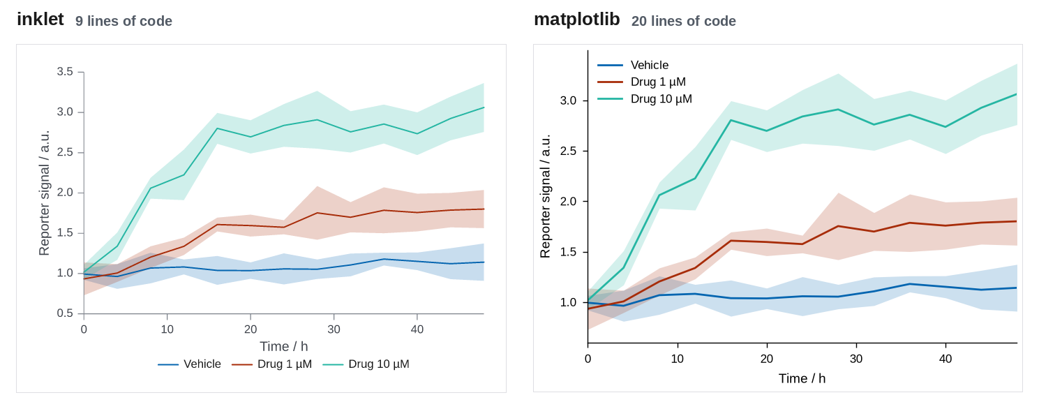
Time course with 95% CI bands: inklet on the left, matplotlib on the right

89 × 63.2 mm · inklet 9 lines, matplotlib 20 lines · inklet report: inklet lint: clean, 0 diagnostics

Where inklet helps: One call draws the means, translucent bands in the series colours, the axis titles and a legend under the plot.

Where matplotlib is better, or inklet needed a workaround: The two scripts are close. matplotlib needs a loop, fill_between and colour matching, about five more lines. The legend placement differs: inklet puts the key under the axes, and matplotlib's legend() places it inside, at the spot with least overlap.

inklet (time_course/inklet_version.py):

import sys
from pathlib import Path

sys.path.insert(0, str(Path(__file__).resolve().parents[1]))

import inklet as i

from data import outputs, time_course

chart = i.line(time_course(), x='time', y='mean', color='condition', error_y='ci',
               xlabel='Time / h', ylabel='Reporter signal / a.u.', xlim=(0, 48))
figure = chart.save(*outputs('time_course', 'inklet'), dpi=200)
print(figure.report())

matplotlib (time_course/matplotlib_version.py):

import sys
from pathlib import Path

sys.path.insert(0, str(Path(__file__).resolve().parents[1]))

import matplotlib
matplotlib.use('Agg')
import matplotlib.pyplot as plt

from data import MM, outputs, time_course

plt.style.use(Path(__file__).resolve().parents[1] / 'journal.mplstyle')
df = time_course()

fig, ax = plt.subplots(figsize=(89 * MM, 63.2 * MM))
for condition, group in df.groupby('condition', sort=False):
    line, = ax.plot(group['time'], group['mean'], label=condition)
    ax.fill_between(group['time'], group['mean'] - group['ci'], group['mean'] + group['ci'],
                    color=line.get_color(), alpha=0.2, linewidth=0)
ax.set_xlim(0, 48)
ax.set_xlabel('Time / h')
ax.set_ylabel('Reporter signal / a.u.')
ax.legend()
for path in outputs('time_course', 'matplotlib'):
    fig.savefig(path)

Grouped bars with error bars and points¶

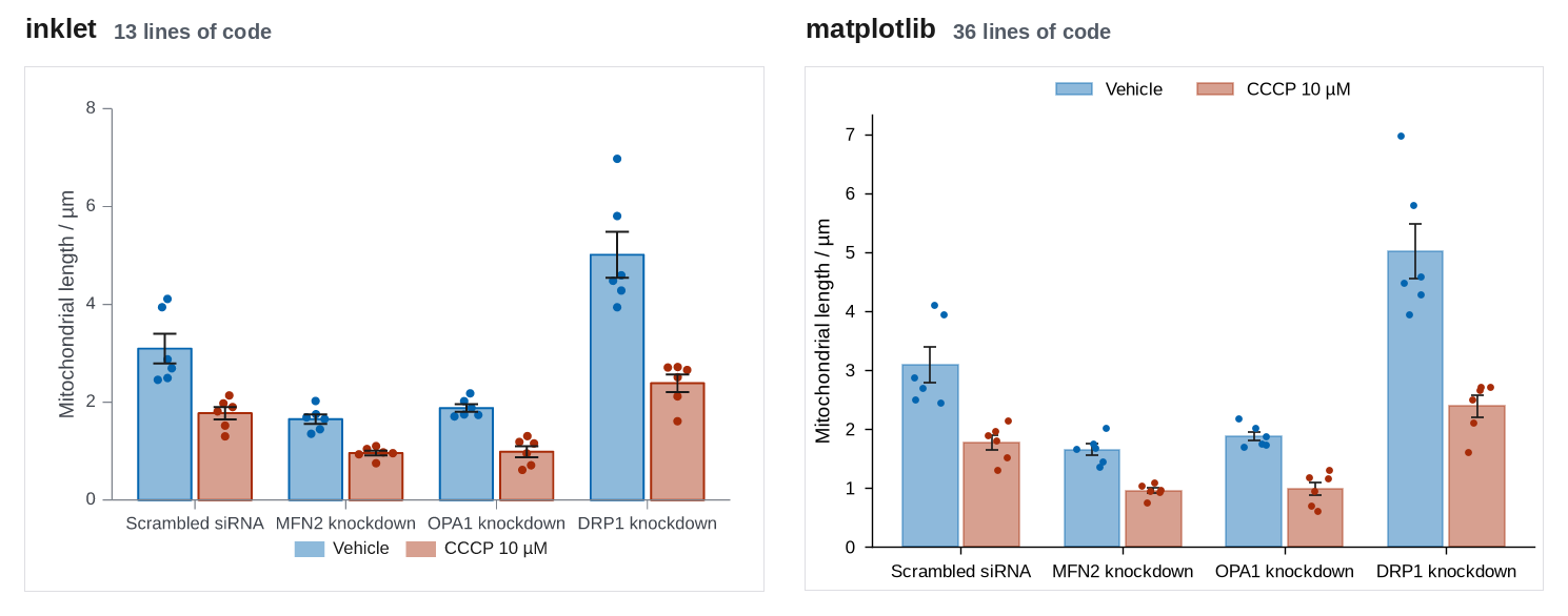
Grouped bars with error bars and points: inklet on the left, matplotlib on the right

89 × 63.2 mm · inklet 13 lines, matplotlib 36 lines · inklet report: inklet lint: clean, 0 diagnostics

Where inklet helps: barplot computes the means and SEMs, dodges the two series, places every observation inside its bar without random jitter, and adds the legend. matplotlib needs manual bar offsets, a groupby for the statistics and a jitter loop.

Where matplotlib is better, or inklet needed a workaround: matplotlib exposes bar width, cap size and point placement directly, and inklet's swarm layout inside each bar has fewer controls.

inklet (grouped_bars/inklet_version.py):

import sys
from pathlib import Path

sys.path.insert(0, str(Path(__file__).resolve().parents[1]))

import inklet as i

from data import mitochondria, outputs

df = mitochondria()
genotypes = list(df['genotype'].unique())
samples = [[df.length[(df.genotype == g) & (df.treatment == t)].tolist() for g in genotypes]
           for t in ('Vehicle', 'CCCP')]

chart = i.chart(ylabel='Mitochondrial length / µm')
chart.barplot(genotypes, samples, name=['Vehicle', 'CCCP 10 µM'])
figure = chart.save(*outputs('grouped_bars', 'inklet'), dpi=200)
print(figure.report())

matplotlib (grouped_bars/matplotlib_version.py):

import sys
from pathlib import Path

sys.path.insert(0, str(Path(__file__).resolve().parents[1]))

import matplotlib
matplotlib.use('Agg')
import matplotlib.pyplot as plt
import numpy as np

from data import MM, mitochondria, outputs

plt.style.use(Path(__file__).resolve().parents[1] / 'journal.mplstyle')
df = mitochondria()
genotypes = list(df['genotype'].unique())
treatments = {'Vehicle': 'Vehicle', 'CCCP': 'CCCP 10 µM'}
stats = df.groupby(['genotype', 'treatment'])['length'].agg(['mean', 'sem'])
rng = np.random.default_rng(0)

fig, ax = plt.subplots(figsize=(89 * MM, 63.2 * MM))
x = np.arange(len(genotypes))
width = 0.38
for k, (treatment, label) in enumerate(treatments.items()):
    color = f'C{k}'
    offset = (k - 0.5) * width
    means = [stats.loc[(g, treatment), 'mean'] for g in genotypes]
    sems = [stats.loc[(g, treatment), 'sem'] for g in genotypes]
    ax.bar(x + offset, means, width * 0.9, color=color, alpha=0.45, edgecolor=color,
           linewidth=0.6, label=label)
    ax.errorbar(x + offset, means, yerr=sems, fmt='none', ecolor='0.1', elinewidth=0.6,
                capsize=2, capthick=0.6)
    for j, g in enumerate(genotypes):
        values = df.length[(df.genotype == g) & (df.treatment == treatment)]
        jitter = rng.uniform(-0.1, 0.1, len(values))
        ax.scatter(x[j] + offset + jitter, values, s=6, color=color, zorder=3, linewidth=0)
ax.set_xticks(x, genotypes)
ax.set_ylabel('Mitochondrial length / µm')
ax.set_ylim(bottom=0)
ax.legend(ncols=2, loc='lower center', bbox_to_anchor=(0.5, 1.0))
for path in outputs('grouped_bars', 'matplotlib'):
    fig.savefig(path)

Dose-response with fitted curves¶

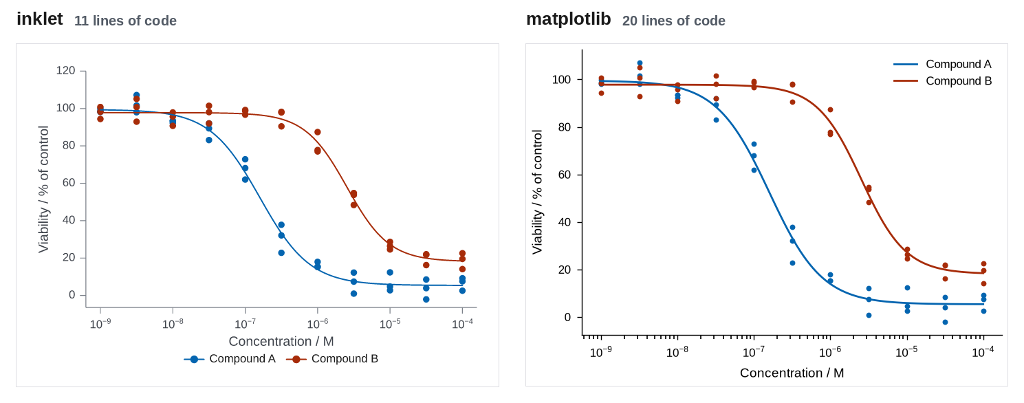
Dose-response with fitted curves: inklet on the left, matplotlib on the right

89 × 63.2 mm · inklet 11 lines, matplotlib 20 lines · inklet report: inklet lint: clean, 0 diagnostics

Where inklet helps: Points and fitted curves of the same compound share a colour and one legend entry without extra code. Both libraries label the log axis as powers of ten.

Where matplotlib is better, or inklet needed a workaround: The two scripts are similar in length, and matplotlib is equally direct. The four-parameter fit is in data.py (no SciPy here), so neither script contains it.

inklet (dose_response/inklet_version.py):

import sys
from pathlib import Path

sys.path.insert(0, str(Path(__file__).resolve().parents[1]))

import inklet as i

from data import dose_response, outputs

points, curves, ec50 = dose_response()
chart = i.scatter(points, x='conc', y='viability', color='compound', size=1.2, xscale='log',
                  xlabel='Concentration / M', ylabel='Viability / % of control')
chart.line(curves, x='conc', y='fit', color='compound')
figure = chart.save(*outputs('dose_response', 'inklet'), dpi=200)
print(figure.report())

matplotlib (dose_response/matplotlib_version.py):

import sys
from pathlib import Path

sys.path.insert(0, str(Path(__file__).resolve().parents[1]))

import matplotlib
matplotlib.use('Agg')
import matplotlib.pyplot as plt

from data import MM, dose_response, outputs

plt.style.use(Path(__file__).resolve().parents[1] / 'journal.mplstyle')
points, curves, ec50 = dose_response()

fig, ax = plt.subplots(figsize=(89 * MM, 63.2 * MM))
for k, (compound, group) in enumerate(points.groupby('compound')):
    fit = curves[curves.compound == compound]
    ax.scatter(group['conc'], group['viability'], s=8, color=f'C{k}', linewidth=0)
    ax.plot(fit['conc'], fit['fit'], color=f'C{k}', label=compound)
ax.set_xscale('log')
ax.set_xlabel('Concentration / M')
ax.set_ylabel('Viability / % of control')
ax.legend()
for path in outputs('dose_response', 'matplotlib'):
    fig.savefig(path)

Violin and strip, four groups¶

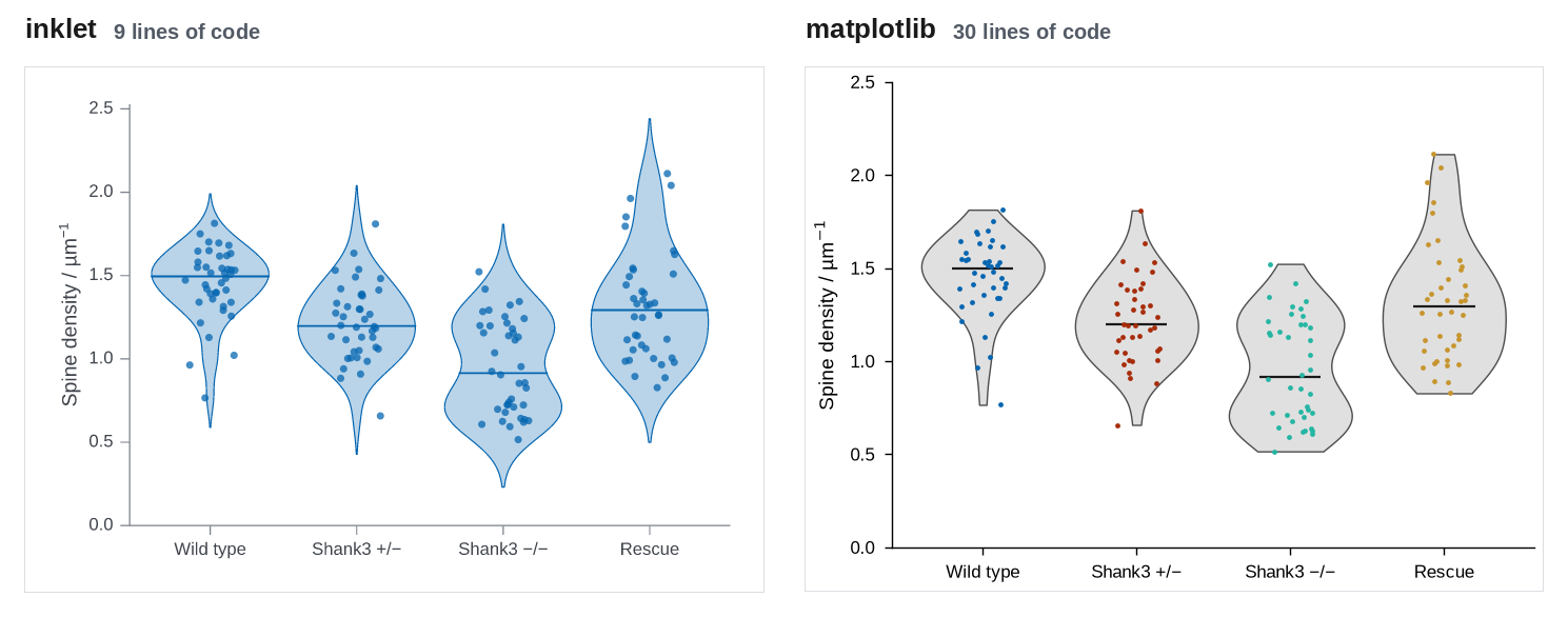
Violin and strip, four groups: inklet on the left, matplotlib on the right

89 × 63.2 mm · inklet 9 lines, matplotlib 30 lines · inklet report: inklet lint: clean, 0 diagnostics

Where inklet helps: violin(points=True) gives the violins, medians and coloured points in one call. matplotlib's violinplot needs seven lines to restyle its bodies and medians, and a loop for the points.

Where matplotlib is better, or inklet needed a workaround: The default density extent differs. inklet extends each violin two bandwidths past the data, like seaborn, and matplotlib stops at the data range. Neither is wrong, but the shapes differ, and inklet's tails can suggest values that were never observed (the Rescue violin reaches 2.45, while the largest observation is 2.11).

inklet (distributions/inklet_version.py):

import sys
from pathlib import Path

sys.path.insert(0, str(Path(__file__).resolve().parents[1]))

import inklet as i

from data import distributions, outputs

chart = i.violin(distributions(), x='genotype', y='density', points=True,
                 xlabel='', ylabel='Spine density / µm^{-1}')
figure = chart.save(*outputs('distributions', 'inklet'), dpi=200)
print(figure.report())

matplotlib (distributions/matplotlib_version.py):

import sys
from pathlib import Path

sys.path.insert(0, str(Path(__file__).resolve().parents[1]))

import matplotlib
matplotlib.use('Agg')
import matplotlib.pyplot as plt
import numpy as np

from data import MM, distributions, outputs

plt.style.use(Path(__file__).resolve().parents[1] / 'journal.mplstyle')
df = distributions()
groups = list(df['genotype'].unique())
samples = [df.density[df.genotype == g].to_numpy() for g in groups]
rng = np.random.default_rng(0)

fig, ax = plt.subplots(figsize=(89 * MM, 63.2 * MM))
parts = ax.violinplot(samples, showmedians=True, showextrema=False, widths=0.8)
for body in parts['bodies']:
    body.set_facecolor('0.88')
    body.set_edgecolor('0.3')
    body.set_linewidth(0.5)
    body.set_alpha(1)
parts['cmedians'].set_color('0.1')
parts['cmedians'].set_linewidth(0.8)
for k, values in enumerate(samples, start=1):
    ax.scatter(k + rng.uniform(-0.15, 0.15, len(values)), values, s=3, color=f'C{k - 1}',
               linewidth=0, zorder=3)
ax.set_xticks(range(1, len(groups) + 1), groups)
ax.set_ylabel('Spine density / µm$^{-1}$')
ax.set_ylim(0, 2.5)
for path in outputs('distributions', 'matplotlib'):
    fig.savefig(path)

Volcano plot with labelled hits¶

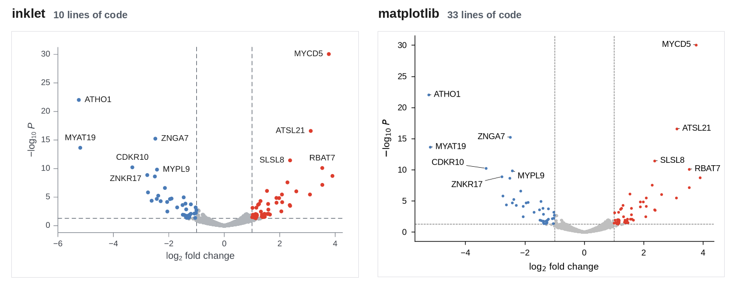
Volcano plot with labelled hits: inklet on the left, matplotlib on the right

89 × 63.2 mm · inklet 10 lines, matplotlib 33 lines · inklet report: inklet lint: 1 info

Where inklet helps: Panel.volcano classifies the genes, draws the threshold rules and labels the ten smallest p-values clear of the points and of each other. In matplotlib, six of the ten labels needed hand-tuned offsets. adjustText, a third-party package, would automate that step but is not installed here.

Where matplotlib is better, or inklet needed a workaround: matplotlib's hand-placed labels can be tuned label by label, but they have to be re-tuned for new data; inklet places them automatically and adds a leader when a neighbour is nearly as close as the labelled point.

inklet (volcano/inklet_version.py):

import sys
from pathlib import Path

sys.path.insert(0, str(Path(__file__).resolve().parents[1]))

import inklet as i

from data import outputs, volcano

df = volcano()
chart = i.chart(xlabel='log_{2} fold change', ylabel='−log_{10} //P//')
chart.volcano(df['log2fc'], df['p'], labels=df['gene'], top=10, size=1.0)
figure = chart.save(*outputs('volcano', 'inklet'), dpi=200)
print(figure.report())

matplotlib (volcano/matplotlib_version.py):

import sys
from pathlib import Path

sys.path.insert(0, str(Path(__file__).resolve().parents[1]))

import matplotlib
matplotlib.use('Agg')
import matplotlib.pyplot as plt
import numpy as np

from data import MM, outputs, volcano

plt.style.use(Path(__file__).resolve().parents[1] / 'journal.mplstyle')
df = volcano()
df['y'] = -np.log10(df['p'])
significant = (df['p'] < 0.05) & (df['log2fc'].abs() >= 1)
classes = {'ns': (~significant, '0.75'),
           'down': (significant & (df['log2fc'] < 0), '#4a7bb7'),
           'up': (significant & (df['log2fc'] > 0), '#dd3d2d')}

fig, ax = plt.subplots(figsize=(89 * MM, 63.2 * MM))
for mask, color in classes.values():
    ax.scatter(df.log2fc[mask], df.y[mask], s=4, color=color, linewidth=0)
for x in (-1, 1):
    ax.axvline(x, color='0.4', linewidth=0.4, linestyle='--', zorder=0)
ax.axhline(-np.log10(0.05), color='0.4', linewidth=0.4, linestyle='--', zorder=0)
nudge = {'ZNKR17': (-14, -6), 'CDKR10': (-16, 4), 'MYPL9': (4, -4), 'ATHO1': (4, 0),
         'MYAT19': (4, 0), 'MYCD5': (-4, 0)}
for _, row in df[significant].nsmallest(10, 'p').iterrows():
    default = (4, 0) if row.log2fc > 0 else (-4, 0)
    offset = nudge.get(row.gene, default)
    ax.annotate(row.gene, (row.log2fc, row.y), xytext=offset, textcoords='offset points',
                ha='left' if offset[0] > 0 else 'right', va='center', fontsize=6,
                arrowprops=dict(arrowstyle='-', linewidth=0.3, shrinkA=0, shrinkB=1))
ax.set_xlabel('log$_2$ fold change')
ax.set_ylabel('$-$log$_{10}$ $P$')
for path in outputs('volcano', 'matplotlib'):
    fig.savefig(path)

Kaplan-Meier curves with number at risk¶

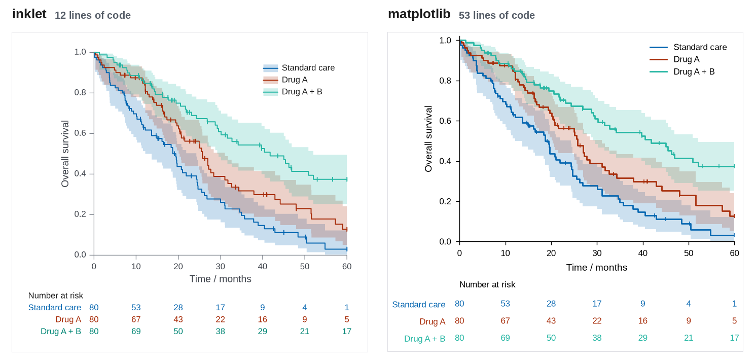
Kaplan-Meier curves with number at risk: inklet on the left, matplotlib on the right

89 × 80 mm · inklet 12 lines, matplotlib 53 lines · inklet report: inklet lint: 2 infos

Where inklet helps: kaplan_meier computes the estimate, the log-log confidence band and the censor ticks, and at_risk() adds a number-at-risk table aligned with the x ticks. matplotlib has no Kaplan-Meier support. 12 of its 53 lines are a hand-written estimator, and the table needs a second axes. With lifelines (not installed here), KaplanMeierFitter and add_at_risk_counts would shorten it considerably.

Where matplotlib is better, or inklet needed a workaround: Both versions blend overlapping confidence bands. matplotlib needs a hand-written estimator (or lifelines) and a second axes for the at-risk table.

inklet (survival/inklet_version.py):

import sys
from pathlib import Path

sys.path.insert(0, str(Path(__file__).resolve().parents[1]))

import inklet as i

from data import outputs, survival

df = survival()
arms = {arm: (group['months'], group['event']) for arm, group in df.groupby('arm', sort=False)}
chart = i.chart(xlabel='Time / months', ylabel='Overall survival', xlim=(0, 60), ylim=(0, 1),
                height=72)
chart.kaplan_meier(arms).legend(corner='ne').at_risk()
figure = chart.save(*outputs('survival', 'inklet'), dpi=200)
print(figure.report())

matplotlib (survival/matplotlib_version.py):

import sys
from pathlib import Path

sys.path.insert(0, str(Path(__file__).resolve().parents[1]))

import matplotlib
matplotlib.use('Agg')
import matplotlib.pyplot as plt
import numpy as np

from data import MM, outputs, survival


def kaplan_meier(time, event, z=1.96):
    """Survival steps with a log-log Greenwood confidence band."""
    times = np.unique(time[event == 1])
    at_risk = np.array([(time >= t).sum() for t in times])
    deaths = np.array([((time == t) & (event == 1)).sum() for t in times])
    s = np.cumprod(1 - deaths / at_risk)
    with np.errstate(divide='ignore', invalid='ignore'):
        var = np.cumsum(deaths / (at_risk * (at_risk - deaths))) / np.log(s) ** 2
        lo, hi = (s ** np.exp(sign * z * np.sqrt(var)) for sign in (1, -1))
    pad = lambda v: np.r_[1.0, v, v[-1]]
    steps = np.r_[0, times, time.max()]
    return steps, pad(s), pad(np.nan_to_num(lo)), pad(np.nan_to_num(hi, nan=1.0))


plt.style.use(Path(__file__).resolve().parents[1] / 'journal.mplstyle')
df = survival()
ticks = np.arange(0, 61, 10)

fig, (ax, risk) = plt.subplots(2, 1, figsize=(89 * MM, 80 * MM), sharex=True,
                               height_ratios=[4, 1])
arms = []
for k, (arm, group) in enumerate(df.groupby('arm', sort=False)):
    time, event = group['months'].to_numpy(), group['event'].to_numpy()
    t, s, lo, hi = kaplan_meier(time, event)
    ax.step(t, s, where='post', color=f'C{k}', label=arm)
    ax.fill_between(t, lo, hi, step='post', color=f'C{k}', alpha=0.2, linewidth=0)
    censored = np.sort(time[event == 0])
    ax.plot(censored, s[np.searchsorted(t, censored, side='right') - 1], '|', color=f'C{k}',
            markersize=3, markeredgewidth=0.6)
    for tick in ticks:
        risk.text(tick, k, (time >= tick).sum(), ha='center', va='center', color=f'C{k}', fontsize=6)
    arms.append(arm)
ax.set_xlim(0, 60)
ax.set_ylim(0, 1.02)
ax.set_xticks(ticks)
ax.tick_params(labelbottom=True)
ax.set_xlabel('Time / months')
ax.set_ylabel('Overall survival')
ax.legend(loc='upper right')
risk.set_ylim(len(arms) - 0.5, -0.5)
risk.set_yticks(range(len(arms)), arms)
for label, k in zip(risk.get_yticklabels(), range(len(arms))):
    label.set_color(f'C{k}')
risk.tick_params(length=0, pad=10, labelbottom=False)
risk.spines[:].set_visible(False)
risk.set_title('Number at risk', loc='left', fontsize=6)
for path in outputs('survival', 'matplotlib'):
    fig.savefig(path)

Correlation heatmap¶

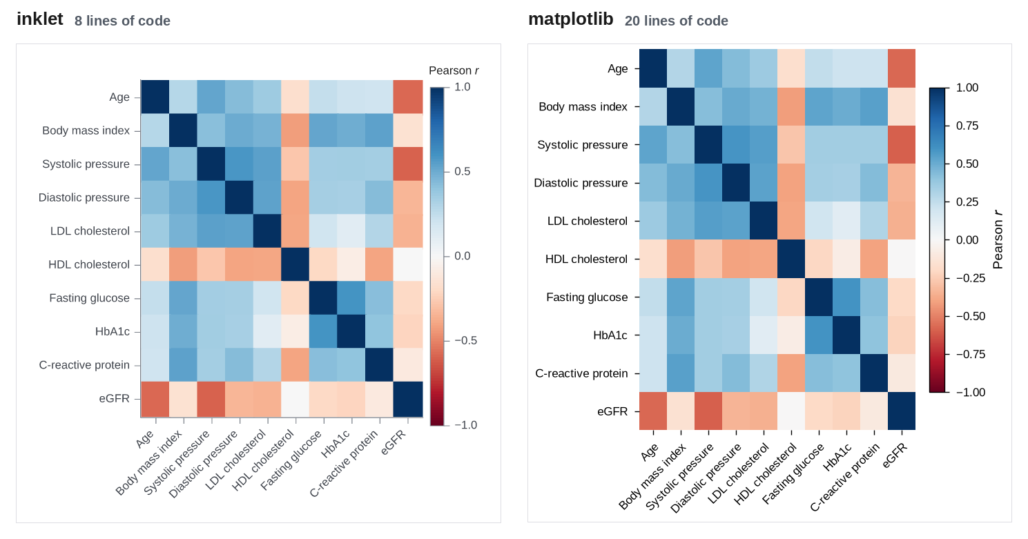
Correlation heatmap: inklet on the left, matplotlib on the right

89 × 88 mm · inklet 8 lines, matplotlib 20 lines · inklet report: inklet lint: clean, 0 diagnostics

Where inklet helps: Row and column labels come from the DataFrame, the rotated x labels are chosen automatically, and colorbar='Pearson //r//' titles the colour bar in the same call.

Where matplotlib is better, or inklet needed a workaround: matplotlib's imshow plus colorbar is about as direct, and most of its extra lines are tick setup.

inklet (heatmap/inklet_version.py):

import sys
from pathlib import Path

sys.path.insert(0, str(Path(__file__).resolve().parents[1]))

import inklet as i

from data import correlation, outputs

chart = i.heatmap(correlation(), palette='rdbu', center=0, height=80, colorbar='Pearson //r//')
figure = chart.save(*outputs('heatmap', 'inklet'), dpi=200)
print(figure.report())

matplotlib (heatmap/matplotlib_version.py):

import sys
from pathlib import Path

sys.path.insert(0, str(Path(__file__).resolve().parents[1]))

import matplotlib
matplotlib.use('Agg')
import matplotlib.pyplot as plt

from data import MM, correlation, outputs

plt.style.use(Path(__file__).resolve().parents[1] / 'journal.mplstyle')
corr = correlation()

fig, ax = plt.subplots(figsize=(89 * MM, 88 * MM))
image = ax.imshow(corr, cmap='RdBu', vmin=-1, vmax=1, aspect='auto')
ax.set_xticks(range(len(corr.columns)), corr.columns, rotation=45, ha='right',
              rotation_mode='anchor')
ax.set_yticks(range(len(corr.index)), corr.index)
ax.spines[:].set_visible(False)
colorbar = fig.colorbar(image, ax=ax, shrink=0.8)
colorbar.set_label('Pearson $r$')
colorbar.outline.set_linewidth(0.5)
for path in outputs('heatmap', 'matplotlib'):
    fig.savefig(path)

Four-panel double-column figure¶

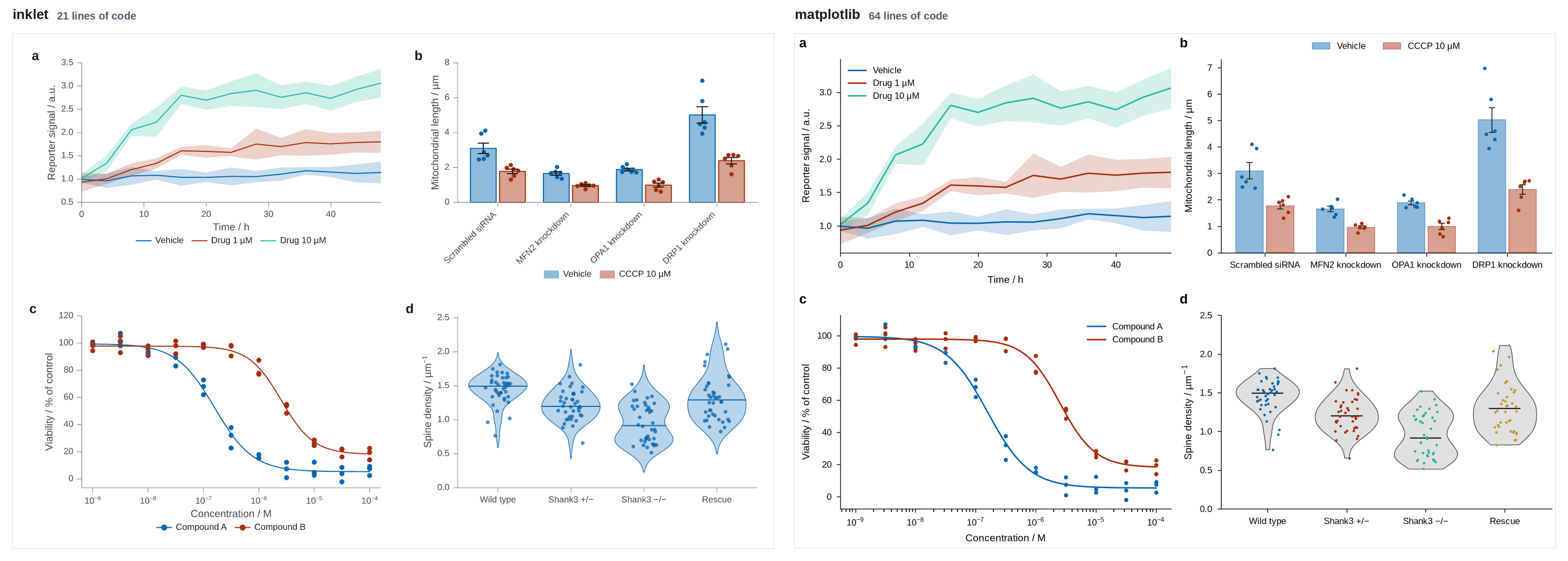
Four-panel double-column figure: inklet on the left, matplotlib on the right

183 × 123.8 mm · inklet 21 lines, matplotlib 64 lines · inklet report: inklet lint: clean, 0 diagnostics

Where inklet helps: The four single-panel chart definitions combine with (a | b) / (c | d) at double-column width, with letters, the same type sizes and aligned axes. The crowded bar labels in panel b are turned automatically.

Where matplotlib is better, or inklet needed a workaround: matplotlib's constrained layout and fig.align_labels() also align the axes. Measured on the PNGs, the y-axis spines of both columns line up in both versions. Panel letters take a ScaledTranslation per axes. The matplotlib line count includes code copied from the single figures. Factoring that into shared functions, as a real project would, makes the composite itself much shorter.

inklet (multi_panel/inklet_version.py):

import sys
from pathlib import Path

sys.path.insert(0, str(Path(__file__).resolve().parents[1]))

import inklet as i

from data import distributions, dose_response, mitochondria, outputs, time_course

course = i.line(time_course(), x='time', y='mean', color='condition', error_y='ci',
                xlabel='Time / h', ylabel='Reporter signal / a.u.', xlim=(0, 48))

cells = mitochondria()
genotypes = list(cells['genotype'].unique())
samples = [[cells.length[(cells.genotype == g) & (cells.treatment == t)].tolist() for g in genotypes]
           for t in ('Vehicle', 'CCCP')]
bars = i.chart(ylabel='Mitochondrial length / µm')
bars.barplot(genotypes, samples, name=['Vehicle', 'CCCP 10 µM'])

points, curves, ec50 = dose_response()
dose = i.scatter(points, x='conc', y='viability', color='compound', size=1.2, xscale='log',
                 xlabel='Concentration / M', ylabel='Viability / % of control')
dose.line(curves, x='conc', y='fit', color='compound')

spread = i.violin(distributions(), x='genotype', y='density', points=True,
                  xlabel='', ylabel='Spine density / µm^{-1}')

figure = ((course | bars) / (dose | spread)).save(*outputs('multi_panel', 'inklet'), dpi=200)
print(figure.report())

matplotlib (multi_panel/matplotlib_version.py):

import sys
from pathlib import Path

sys.path.insert(0, str(Path(__file__).resolve().parents[1]))

import matplotlib
matplotlib.use('Agg')
import matplotlib.pyplot as plt
import numpy as np
from matplotlib.transforms import ScaledTranslation

from data import MM, distributions, dose_response, mitochondria, outputs, time_course

plt.style.use(Path(__file__).resolve().parents[1] / 'journal.mplstyle')
rng = np.random.default_rng(0)
fig, axes = plt.subplots(2, 2, figsize=(183 * MM, 123.8 * MM))
(ax_a, ax_b), (ax_c, ax_d) = axes

course = time_course()
for condition, group in course.groupby('condition', sort=False):
    line, = ax_a.plot(group['time'], group['mean'], label=condition)
    ax_a.fill_between(group['time'], group['mean'] - group['ci'], group['mean'] + group['ci'],
                      color=line.get_color(), alpha=0.2, linewidth=0)
ax_a.set(xlim=(0, 48), xlabel='Time / h', ylabel='Reporter signal / a.u.')
ax_a.legend()

cells = mitochondria()
genotypes = list(cells['genotype'].unique())
stats = cells.groupby(['genotype', 'treatment'])['length'].agg(['mean', 'sem'])
x = np.arange(len(genotypes))
for k, (treatment, label) in enumerate({'Vehicle': 'Vehicle', 'CCCP': 'CCCP 10 µM'}.items()):
    offset = (k - 0.5) * 0.38
    means = [stats.loc[(g, treatment), 'mean'] for g in genotypes]
    sems = [stats.loc[(g, treatment), 'sem'] for g in genotypes]
    ax_b.bar(x + offset, means, 0.34, color=f'C{k}', alpha=0.45, edgecolor=f'C{k}',
             linewidth=0.6, label=label)
    ax_b.errorbar(x + offset, means, yerr=sems, fmt='none', ecolor='0.1', elinewidth=0.6,
                  capsize=2, capthick=0.6)
    for j, g in enumerate(genotypes):
        values = cells.length[(cells.genotype == g) & (cells.treatment == treatment)]
        ax_b.scatter(x[j] + offset + rng.uniform(-0.1, 0.1, len(values)), values, s=6,
                     color=f'C{k}', zorder=3, linewidth=0)
ax_b.set_xticks(x, genotypes)
ax_b.set(ylabel='Mitochondrial length / µm', ylim=(0, None))
ax_b.legend(ncols=2, loc='lower center', bbox_to_anchor=(0.5, 1.0))

points, curves, ec50 = dose_response()
for k, (compound, group) in enumerate(points.groupby('compound')):
    fit = curves[curves.compound == compound]
    ax_c.scatter(group['conc'], group['viability'], s=8, color=f'C{k}', linewidth=0)
    ax_c.plot(fit['conc'], fit['fit'], color=f'C{k}', label=compound)
ax_c.set(xscale='log', xlabel='Concentration / M', ylabel='Viability / % of control')
ax_c.legend()

spread = distributions()
groups = list(spread['genotype'].unique())
samples = [spread.density[spread.genotype == g].to_numpy() for g in groups]
parts = ax_d.violinplot(samples, showmedians=True, showextrema=False, widths=0.8)
for body in parts['bodies']:
    body.set(facecolor='0.88', edgecolor='0.3', linewidth=0.5, alpha=1)
parts['cmedians'].set(color='0.1', linewidth=0.8)
for k, values in enumerate(samples, start=1):
    ax_d.scatter(k + rng.uniform(-0.15, 0.15, len(values)), values, s=3, color=f'C{k - 1}',
                 linewidth=0, zorder=3)
ax_d.set_xticks(range(1, len(groups) + 1), groups)
ax_d.set(ylabel='Spine density / µm$^{-1}$', ylim=(0, 2.5))

for ax, letter in zip(axes.flat, 'abcd'):
    ax.text(0, 1, letter, transform=ax.transAxes + ScaledTranslation(-28 / 72, 6 / 72, fig.dpi_scale_trans),
            fontsize=9, fontweight='bold', va='bottom')
fig.align_labels()
for path in outputs('multi_panel', 'matplotlib'):
    fig.savefig(path)

Lines of code¶

Figure	inklet	matplotlib	inklet report
Time course with 95% CI bands	9	20	`inklet lint: clean, 0 diagnostics`
Grouped bars with error bars and points	13	36	`inklet lint: clean, 0 diagnostics`
Dose-response with fitted curves	11	20	`inklet lint: clean, 0 diagnostics`
Violin and strip, four groups	9	30	`inklet lint: clean, 0 diagnostics`
Volcano plot with labelled hits	10	33	`inklet lint: 1 info`
Kaplan-Meier curves with number at risk	12	53	`inklet lint: 2 infos`
Correlation heatmap	8	20	`inklet lint: clean, 0 diagnostics`
Four-panel double-column figure	21	64	`inklet lint: clean, 0 diagnostics`
Total	93	276

Shared files are not counted above: data.py (135 lines, used by both) and journal.mplstyle (23 lines, matplotlib only).

Line counts measure typing, not quality. The bigger differences are in the domain plots. matplotlib needed a hand-written Kaplan-Meier estimator and hand-placed volcano labels, and inklet has both built in. For the plain charts (lines, scatter, heatmap) the matplotlib code is short and direct, and both libraries produce clean figures at print size.