

On this page
inklet cookbook
Recipes for the shapes that come up in a real figure and are not obvious from
the reference. Every block here is executed by tests/test_cookbook.py, and
most of them assert a clean lint.
This is the direct drawing reference: diagrams and panels keep their authored physical sizes. For a page that follows data edits and resizes its plots, start with the first figure tutorial and the authoring model. Use this cookbook for individual drawing techniques inside either workflow. The examples use illustrative data unless their source is stated; sections that need optional tools identify them locally.
Each recipe starts from:
import inklet

TH = inklet.use_theme("nature")
Fit content to a column
inklet.figure(width=...) sets the page. It does not constrain what you put on
it: content that does not fit is reported as OFF_CANVAS, not shrunk. When you
have a column budget -- 89 mm for one column, 178 mm for two -- and content
whose size you will only know after the text is shaped, inklet.fit solves it.
BODY = ("Participants were assessed for eligibility between March 2021 and "
        "November 2022 at four centres.")

card = inklet.fit(lambda w: inklet.box(inklet.text(BODY, width=w)), width=52)
assert card.width == 52.0
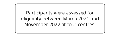
Rendered from the code above.
The quantity being solved for can be a wrap width, plot area, radius, or font
size. fit only compares what comes back against
the target. Because text wraps in whole words the measurement moves in jumps,
so fit returns the widest build that still fits and pads the remainder;
pass exact=False for the content's own size instead.
If the recipe has a minimum of its own -- a legend, a word that will not break
-- fit raises and names that minimum, which is the number you actually need.
A flow with a branch off the spine
The most common shape in a methods figure: a vertical spine, with something
hanging off it between two boxes. The join is a zero-size spacer standing in
the stack, which gives the branch somewhere to start that moves when the layout
moves.
top = inklet.box("Assessed for eligibility (n = 1,204)", width=54)
junction = inklet.spacer(0.01, 0.01)
bottom = inklet.box("Randomised (n = 816)", width=54)
aside = inklet.box("Excluded (n = 388)", width=36)

spine = inklet.vstack([top, junction, bottom], gap=9)
body = inklet.hstack([spine, aside], gap=10, align="center")

fig = inklet.figure(width=120)
fig.add(body)
fig.link(top, bottom, through=[junction])
fig.link(junction.at("center"), aside, route="orthogonal")

assert fig.lint() == []
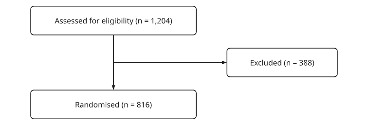
Rendered from the code above.
Two settings are required. through=[junction] tells the spine's arrow that
passing over the join is not a collision. And the branch starts at
junction.at("center"), not at junction: a spacer draws nothing, so
there is no outline for a link to clip against, and aiming at the node itself
produces LINK_UNCLIPPED. An anchor supplies a position rather than a clipping
outline, which is appropriate for an invisible join.
A graph that lays itself out
For flows with about a dozen or more boxes, manual stacking requires repeated
gap and placement changes. inklet.graph takes the boxes and edges and computes
ranks, order within each rank, edge corridors, and physical positions.
STEPS = {
    "raw": "raw traces", "ref": "template", "reg": "register",
    "seg": "segment", "qc": "QC", "fit": "fit model",
    "stat": "statistics", "fig": "figure",
}
boxes = {key: inklet.box(text, width=18) for key, text in STEPS.items()}
edges = [
    ("raw", "reg"), ("ref", "reg"), ("reg", "seg"), ("seg", "qc"),
    ("qc", "fit"), ("fit", "stat"), ("stat", "fig"), ("seg", "fig"),
]

pipeline = inklet.graph(boxes, edges, direction="down")

fig = inklet.figure(width=120)
pipeline.add_to(fig)

assert pipeline["seg"] is boxes["seg"]     # the very box, still yours
assert [d for d in fig.lint() if d.severity == "error"] == []
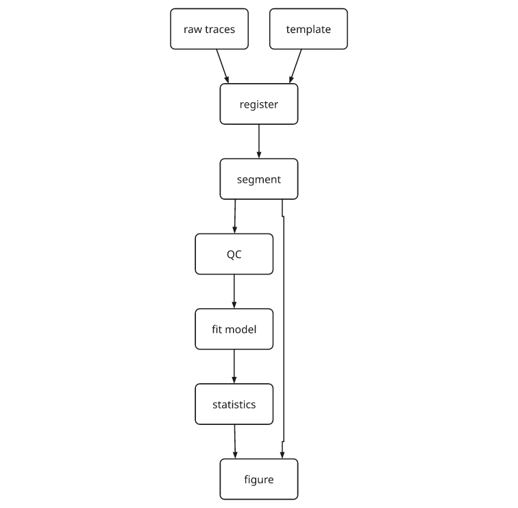
Rendered from the code above.
graph returns a Graph, not a Diagram, because a graph is two things: a
laid-out picture and a set of arrows that can only be routed once the picture
has settled. add_to(fig) does both -- it adds pipeline.diagram and then
calls fig.link for every edge, so labels are shaped by the figure's theme.
pipeline.diagram on its own stacks, pads and frames like anything else.
The layout wraps the boxes rather than rewriting them, so every handle you
already hold still resolves: boxes["seg"] can be linked to, annotated, or
aimed at from outside the graph after the fact.
Four layouts, and the choice is about what the graph is:
"layered"(the default) for directed structures such as pipelines, workflows and CONSORT diagrams. It assigns nodes to ranks."tree"for a real hierarchy: a taxonomy, a decision tree, a file layout. Parents sit centred over their children and subtrees never interleave."force"for an undirected network with no flow to it -- connectivity, co-occurrence. The layout is deterministic and does not require a seed."circular"for a small dense graph where every node should be equally visible.
Edges take a third item: a string is a label, a mapping is keywords for
fig.link.
labelled = inklet.graph(
    {"a": inklet.box("acquire"), "b": inklet.box("archive")},
    [("a", "b", "2 TB/day")],
)
assert labelled.edges[0].label is not None
A self-loop or a second edge between the same two boxes raises because both
would be represented by one line with two arrowheads. Draw a loop yourself with
inklet.arc, or merge the two edges and put both labels on one.
Which way an orthogonal arrow bends
route="orthogonal" selects an axis-aligned route. The elbow is decided before
clipping.
- The connector leaves along whichever axis separates the two centres most.
- If the two shapes are clear of each other on that axis, it leaves and arrives along it, creating a Z route.
- If they overlap on that axis there is no corridor, so it turns once and arrives on the minor axis, creating an L route.
So a bend you did not expect usually means the dominant axis is not the one you had in mind. Moving the two shapes changes the answer; so does an extra millimetre of stack gap.
Boxes that match each other's size
grid equalises cells, not the children inside them, so two boxes of
different text end up different sizes in the same rank. Measure once, then
rebuild at the maximum.
def matched(*contents, gap=3.0):
    """Siblings at one size, so a rank of them reads as a rank."""
    first = [inklet.box(c) for c in contents]
    width = max(b.width for b in first)
    height = max(b.height for b in first)
    return inklet.hstack([inklet.box(c, width=width, height=height) for c in contents],
                      gap=gap, align="top")

arms = matched("Allocated to intervention (n = 408)",
               "Allocated to usual care (n = 408)")
assert arms.height < 12.0

Rendered from the code above.
A hole in a grid
grid is row-major over a flat list and has no notion of an empty cell. A
spacer is the empty cell; a bare Diagram() is not, because an empty node
occupies nothing and trips EMPTY_DIAGRAM.
cells = [inklet.box("a"), inklet.spacer(0.01, 0.01), inklet.box("c"), inklet.box("d")]
sparse = inklet.grid(cells, cols=2, col_gap=4, row_gap=4)
assert sparse.height > sparse.width
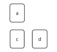
Rendered from the code above.
Several groups, one set of coordinates
Everything in inklet.draw is rewritten to sit on its own origin -- that is what
lets a curve stack and rotate like a box -- and it remembers where the author's
(0, 0) went. inklet.drawn(items) reads that memory back: the group comes out in
the coordinates it was typed in, so the geometry, the markers riding on it and
the labels hung off it stay in one frame. overlay(..., align="origin") is the
combinator that respects it; the plain overlay aligns bounding boxes, which
is what it is for.
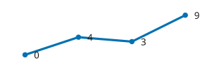
track = [(0, 0), (12, -4), (24, -3), (36, -9)]

line = inklet.drawn(inklet.polyline(track, stroke=TH.accent, stroke_width=TH.thick))
dots = inklet.drawn([(p, inklet.marker("circle", 1.2, fill=TH.accent)) for p in track])
tags = inklet.drawn([((x + 2.0, y), inklet.label(f"{-y}")) for x, y in track],
                 anchor="w")

chart = inklet.overlay([line, dots, tags], align="origin")
assert chart.bbox.width > 36          # the labels hang off the right-hand end
assert inklet.lint(chart) == []
Rendered from the code above.
Without it, each group is centred on its own bounding box. The labelled group is the widest, so the three groups are offset by half the width difference and the drawing is out of register.
loose = inklet.overlay([line.copy(), dots.copy(), tags.copy()])
assert loose.bbox.width < chart.bbox.width
inklet.drawn(items) is inklet.place(items, origin=(0, 0)) under the name that
says which of the two you meant, and place itself puts a bare diagram --
one that is not in a (point, diagram) pair -- back where it was drawn. The
stacks take align="origin" too, on their cross axis: across a row of
sparklines drawn in data coordinates it lines up their y = 0, the way
align="baseline" lines up type.
Cutting a shape to a window
For complete paint cropping, including images, glyphs and smooth filled curves,
use inklet.window(). The geometric operation below changes the
remaining shape and its measured extent.
inklet.clip cuts geometry rather than emitting an SVG clipPath, so the result
measures right -- bbox shrinks, and a stack packs against the ink that is
actually left. The region is a inklet.Rect or a ring of points, convex, and
expressed in the coordinates of whoever holds the node -- which is a reason to
build the thing being cut with inklet.drawn.
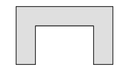
outline = [(0, 0), (30, 0), (30, 18), (24, 18), (24, 6), (6, 6), (6, 18), (0, 18)]
part = inklet.drawn(inklet.polygon(outline, fill=inklet.mix(TH.ink, TH.paper, 0.86),
                             stroke=TH.ink, stroke_width=TH.stroke))

arms = inklet.clip(part, inklet.Rect(-1, 8, 31, 19))
assert inklet.to_svg(arms).count("Z") == 2      # two rings, not one bridged ring
Rendered from the code above.
A window across both arms of that U leaves two separate pieces. Assert this because the textbook algorithm (Sutherland-Hodgman) answers with one ring joined by a zero-width bridge along the cut: right as a nonzero fill and wrong as everything else -- the bridge is stroked, it is a hole under the even-odd rule, and it is not the outline anything downstream measures.
A formula with subscripts
_{...} lowers and ^{...} raises. The braces are the whole of the syntax,
so an underscore in a gene name or a caret in a unit is never touched, and
there is no escaping step. The rest of the markup -- bold, italic, colour --
is in the next recipe, and composes with these.
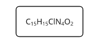
formula = inklet.box("C_{15}H_{15}ClN_{4}O_{2}")
assert inklet.to_svg(formula).count('<tspan') == 8   # C 15 H 15 ClN 4 O 2
assert formula.width < inklet.box("C15H15ClN4O2").width

ion = inklet.text("Ca^{2+} influx, ΔF/F_{0}")
assert ion.prim.lines[0].runs                 # small, shifted runs
assert inklet.text("file_name or m^-1").prim.lines[0].runs == ()
Rendered from the code above.
The scripts are shaped in the same face at 65% of the size and measured like
everything else, so a box around a formula fits it, a wrapped paragraph
breaks in the right places, and text_to_paths outlines the same glyphs the
SVG backend draws.
Inline bold, italic and colour
A caption can contain bold panel letters and an italic species name inside a
justified paragraph. A separate
diagram per phrase cannot be justified into the paragraph around it. Put the
markup in the string; inklet.text, inklet.label, inklet.title and
a box's label all read it.
| written | gives |
|---|---|
**bold** |
the family's real bold face |
//italic// |
the family's real italic face |
{accent\|text} |
a theme token -- ink, muted, accent, paper, grid, series0... |
{#c1121f\|text} |
or any literal fill |
_{sub}, ^{super} |
as in the recipe above |
\*, \/, \{, \_, \^, \|, \\ |
that character, literally |
The delimiters are doubled to avoid ambiguity. A lone * is the adsorbed-species
prefix in electrochemistry captions (*CO, *OH) and a
lone / is in the middle of every URL, so Markdown's single-character
spellings would consume adjacent paragraph text. Two rules make the rest
predictable: each opener takes the nearest matching closer, so delimiters
never cross, and a delimiter with no partner is ordinary text, so
half-typed markup shows up as itself instead of eating what follows it.
caption = inklet.text(
    "**(a)** //Operando// FTIR: the *CO band grows in before "
    "C_{2}H_{4} appears, at 200 mA cm^{−2}.",
    width=70, align="justify")

first = caption.prim.lines[0]
assert len({run.font_path for run in first.runs}) == 3   # regular, bold, italic
assert "**" not in first.text            # the markup never reaches the page
assert "*CO" in first.text               # and a lone star is not markup

keyed = inklet.text("the {accent|measured} curve and the {#c1121f|fit}")
assert [run.fill for run in keyed.prim.lines[0].runs if run.fill] == \
    ["#0072b2", "#c1121f"]

# A string that must arrive exactly as typed.
raw = "50/50 in *CO_{2}"
assert inklet.text(raw, markup=False).prim.lines[0].text == raw
assert inklet.text(inklet.escape_markup(raw)).prim.lines[0].text == raw

Rendered from the code above.
Bold and italic are faces, not a synthetic slant or a double strike: they are found by the same fontconfig lookup that finds the regular one, each run is shaped in its own face, and those run advances are what the wrapper measures. So a bold phrase takes the width it will actually draw at, a justified column still lands exactly on its edge, and a bold phrase may break across a line -- the marks are carried per character, so the wrapper is free to cut through the middle of one.
Colour is per run rather than per node for the same reason: {accent|this
curve} inside a sentence cannot be a second text node without giving up the
justification around it.
Text built from data -- a file path, a label out of a CSV -- should take
markup=False, or go through inklet.escape_markup(s) if it has to sit inside a
caption that does use markup.
A list with hanging indents
A inklet.text block wraps, but it has no notion of a list: every line of a
wrapped paragraph starts at the same margin. Stack one text node per item and
pad each one on the left.
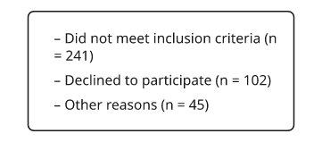
def bullets(*items, indent=1.6, gap=1.0, width=40.0):
    return inklet.vstack([inklet.pad(inklet.text(f"– {i}", width=width, align="left"),
                               0, 0, 0, indent)
                       for i in items], gap=gap, align="left")

reasons = inklet.box(bullets("Did not meet inclusion criteria (n = 241)",
                          "Declined to participate (n = 102)",
                          "Other reasons (n = 45)"))
assert reasons.width > 0
Rendered from the code above.
The gap between items is leading, not clearance, and CROWDING knows the
difference: lines of type stacked in one container are exempt from the
millimetre floor that applies between objects.
A shaded span on a plot
Panel gives you line, marks, place, under and over, but no shaded
region. Map the corners through the scales and draw a polygon underneath.
(inklet.plot.band is a scale constructor, not this.)
p = inklet.panel(60, 20, x=(0, 52), y=["Usual care", "Intervention"])
y = p.point(0, "Intervention").y
half = 3.0

p.under(inklet.polygon(((p.point(0, "Intervention").x, y - half),
                     (p.point(24, "Intervention").x, y - half),
                     (p.point(24, "Intervention").x, y + half),
                     (p.point(0, "Intervention").x, y + half)),
                    fill=inklet.mix(TH.ink, TH.paper, 0.86), stroke="none"))

p.line(((0, "Intervention"), (52, "Intervention")))
p.line(((0, "Usual care"), (52, "Usual care")))
p.marks(inklet.marker("circle", 1.3),
        [(w, "Intervention") for w in (0, 12, 24, 40, 52)])
p.axis("left", spine=False, tick_size=0, tick_pad=2.2)
p.axis("bottom", ticks=[0, 12, 24, 40, 52], label="Weeks from randomisation")

schedule = p.build()
assert inklet.lint(schedule) == []
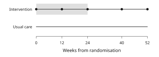
Rendered from the code above.
A band scale puts categories[0] at the low end of the range, and a
panel's y axis runs upward from the bottom of the plot area -- so the first
category is the bottom track. List them in the order you want to read them
upward.
Note every corner above goes through p.point(...) first. under and
over are the two methods on Panel that take panel coordinates --
millimetres from the centre of the plot area -- rather than data. line,
marks, place and point all speak data and map it for you; under and
over take a finished diagram and set only its paint order, so there is
nothing left for them to map. Passing a datum straight in is silent and wrong:
on a panel spanning -1 to 3.5, 0.0 is not t = 0, it is the middle of
the axis, and a rule drawn in the wrong place is a rule drawn perfectly well
as far as the linter is concerned.
p = inklet.panel(60, 20, x=(-1, 3.5), y=(0, 1))
at = p.x.map(0.0)                       # t = 0, in millimetres
p.over(inklet.polyline([(at, p.area.y0), (at, p.area.y1)],
                    stroke=TH.ink, stroke_width=TH.stroke))
assert abs(at - p.area.x0 - 60 / 4.5) < 1e-9    # one second in from the left
assert at != 0.0                                # 0.0 would have been t = 1.25
assert abs(p.x.map(1.25)) < 1e-9                # ...which is the axis midpoint
A greyscale-safe fill
A theme gives you five named colours and a categorical palette, not a tint
ramp. A fill that survives greyscale is a tint of the ink, which is mix.
pale = inklet.mix(TH.ink, TH.paper, 0.86)   # 86% of the way to the paper
mid = inklet.mix(TH.ink, TH.paper, 0.55)
assert inklet.contrast_ratio(TH.ink, pale) > 4.5
inklet.lighten and inklet.darken are the one-colour versions.
A series colour you can read
A categorical palette is built for area. The inklet palette's yellow is 1.26:1 on
white and its sky blue 1.9:1 -- fine as a bar, unreadable as the word that
names the bar. TH.text_color(i) is the same colour darkened along its own
hue until it clears 4.5:1, so it still matches the swatch beside it.
swatch = inklet.polygon(((0, 0), (3.2, 0), (3.2, 1.7), (0, 1.7)),
                     fill=TH.color(4), stroke="none")
name = inklet.label("Vehicle", text_fill=TH.text_color(4))

assert inklet.contrast_ratio(TH.color(4), TH.paper) < 4.5       # the fill, as type
assert inklet.contrast_ratio(TH.text_color(4), TH.paper) >= 4.5
assert inklet.lint(inklet.hstack([swatch, name], gap=1.4)) == []
Three neighbours, three different questions:
TH.color(i)is the published value. Use it for the fill and nothing else.TH.ink_color(i)blends towards the theme's ink until it clears 3:1, the threshold for a rule or an arrowhead. A small drift towards grey is invisible at 0.25 mm, and blending is the cheaper answer there.TH.text_color(i)holds the hue and moves the lightness until it clears 4.5:1, the threshold for type. At that distance a blend has arrived at something closer to grey than to the series, which is why this one exists.
inklet.readable(color, on) is the same search on any two colours, and
TH.text_on(fill) is the other question entirely -- ink or paper, whichever
survives on top of a filled box.
chip = inklet.box(inklet.label("n = 214", text_fill=TH.text_on(TH.color(0))),
               fill=TH.color(0), stroke="none")
assert inklet.lint(chip) == []
A key that is not palette swatches
inklet.legend is built around a categorical palette. When a key explains a
shaded span and a marker rather than a series, build it from the same components
as the figure so its symbols and styling match.
swatch = inklet.polygon(((0, 0), (3.2, 0), (3.2, 1.7), (0, 1.7)),
                     fill=inklet.mix(TH.ink, TH.paper, 0.86), stroke=TH.ink,
                     stroke_width=TH.stroke)

key = inklet.vstack([
    inklet.hstack([swatch, inklet.label("Intervention period")], gap=1.4),
    inklet.hstack([inklet.marker("circle", 1.3), inklet.label("Assessment visit")], gap=1.4),
], gap=1.4, align="left")

assert inklet.lint(key) == []
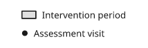
Rendered from the code above.
Reading the linter
fig.report() is the formatted version of fig.lint(), and both take the
thresholds as keywords. The defaults are house style, not your journal's:
fig = inklet.figure(width=89)
fig.add(inklet.vstack([inklet.box("read"), inklet.box("write")], gap=6))

strict = fig.lint(min_font_pt=6.0, min_clearance_mm=1.5, max_stroke_widths=3)
assert strict == []
The severities distinguish findings that require different kinds of review:
- error — examples include text below the minimum size (
TINY_TEXT), overflowing text (TEXT_OVERFLOW), off-page content (OFF_CANVAS), a path crossing text (PATH_CROSSES), and collapsed links (LINK_COLLAPSED). - warning — examples include unclipped links (
LINK_UNCLIPPED) and paths crossing drawings (PATH_CROSSES). Inspect their geometry and placement. - info — review findings such as
CROWDINGandINCONSISTENT_STROKEin context; some figures intentionally use close marks or varied line weights.
Six rules read the relationship between two things rather than one node on its own. Their names identify checks that other rules do not perform:
PATH_CROSSES-- a leader, an annotation arrow or any hand-drawn stroke running through a drawing on its way somewhere else.OVERLAPcompares areas and a stroke has none, so this was invisible until now: it cuts the stroke against the real outline, not the bounding box, and it knows the difference between arriving at something and passing through it.KEY_MISMATCH-- the colorbar or legend does not describe the marks in the panel beside it. The classic is a key written from the list of categories rather than from the categories actually plotted: a swatch for a colour that is drawn nowhere collides with nothing and lints clean without this.COINCIDENT_SHAFT-- two links running along the same line, one hidden under the other. Aim one of them at an anchor rather than at the shape.LINK_CROSSES_LINK-- two connectors crossing each other. Aninfo, because a graph of any density has some; a warning when the crossing falls under a label plate, where the reader cannot follow either line through it. Fix it by reordering the nodes, or withroute="avoid"on one of the two.LABEL_COVERS_SHAFT-- a link's own label plate over its own elbow, leaving a stub of line and an arrowhead that belongs to nothing.TEXT_FILL_IGNORED--fill=on a text node. Glyph colour is thetext_fill=channel;filllands on the group around the type.
One rule depends on an optional package. LOW_CONTRAST averages the pixels
under a caption when the backdrop is a photograph, which needs Pillow. Without
it that one case is skipped rather than guessed at -- white type on a dark
micrograph is never reported against the page colour it is nowhere near.
Review each finding against the rendered figure. The API reference lists all diagnostic codes.
Saying that two things touch on purpose
Some drawings are made of parts that share an edge: Sankey ribbons meeting at a
node, the arcs of a chord ring, a ball-and-stick molecule, a stacked bar. There
OVERLAP and CROWDING are asking the author to break the picture, and there
is no clearance number that tells the difference -- the ribbons touch at 0.00mm
and so does a slipped label.
inklet.abutting(kind) is the declaration, and it works like inklet.encoded(kind):
it marks the kind of the node you put it on -- any place, drawn or leaf
that takes a kind= -- and the two rules skip any pair of items inside that
subtree. It is scoped and symmetric: the claim is that the parts of this thing
touch each other, not that this thing may touch whatever is next to it, so the
ring is still answerable to the key beside it.
left = inklet.box("in", width=20, height=10)
right = inklet.box("out", width=20, height=10).translated(20.4, 0)

assert [d.code for d in inklet.lint(inklet.place([left, right]))] == ["CROWDING"]

declared = inklet.place([left, right], kind=inklet.abutting("ribbons"))

assert inklet.lint(declared) == []
inklet.three.scene declares itself: the parts of one model are one object's
geometry and were never a finding. So is a Panel.draw shape against another
one in the same panel -- both are where the scales put them.
A matrix with a key that cannot disagree with it
Panel.matrix colours one cell per value. The main requirement is that the key
beside it describes the same mapping.
KEY_MISMATCH catches half of that for you -- a bar and a matrix on different
ramps -- but two scales on the same ramp with different domains draw exactly
the same colours, so they lint clean despite having different domains. Build
one scale object and hand it to both.
import math

VALUES = [[math.sin(r / 3.0) * math.cos(c / 5.0) * 1.4 + 0.6
           for c in range(30)] for r in range(12)]

heat_scale = inklet.symlog((-0.8, 2.0), linthresh=0.5)     # built once
shades = inklet.ramp("tol-ylorbr")

p = inklet.panel(60, 24, x=(0, 30), y=(12.5, 0.5))
p.matrix(VALUES, ramp=shades, scale=heat_scale)
p.outline()
p.axes(x="column", y="row")

key = inklet.colorbar(shades, domain=(-0.8, 2.0), scale=heat_scale,
                   length=24, thickness=2.4, label="value",
                   ticks=[-0.8, 0.0, 0.5, 2.0], thin=False,
                   format=lambda v: f"{v:g}")

heatmap = inklet.hstack([p.build(), key], gap=6, align="center")
assert inklet.lint(heatmap) == []
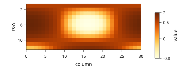
Rendered from the code above.
Three things that are easy to get wrong and are handled for you. Cells overlap
their neighbours slightly, so no pale antialiasing seam draws a grid over the
picture. They use kind="mark", so 360 cells do not produce 700 CROWDING findings.
And values[0] is the top row, which is what a reader expects of a matrix
and the opposite of what a y axis does -- hence y=(12.5, 0.5), counting down.
Naming the ticks matters more here than on a linear axis: the automatic choice
picks round numbers in value space, and on a symlog key that leaves the
baseline and the maximum unlabelled. thin=False keeps every one you asked
for.
One node per cell. A 40 x 90 matrix is 3,600 rectangles and about a
megabyte of SVG. This is suitable for an editable figure but inefficient for a
photograph; use inklet.image for photographic content.
Telling the linter a position is data
CROWDING measures the gap between two things and asks whether a reader can
tell them apart. That question only makes sense when a layout put them there.
When the position came from the data -- a scatter, a heatmap cell, a facet of a
mesh -- the gap is what the measurement says, and "add 0.7mm of separation"
would misrepresent the figure.
inklet.plot marks and inklet.three facets already declare this, so they are
exempt from each other and you will never see it. Anything you compute and
draw yourself does not, because a polygon is a polygon. Say so with
kind="mark":
import math

xs = [(i / 24.0) * 6.0 - 3.0 for i in range(25)]
lobe = [(x, 1.6 * math.exp(-x * x)) for x in xs]
outline = [(x, y) for x, y in lobe] + [(x, -y) for x, y in reversed(lobe)]

p = inklet.panel(50, 30, x=(-3, 3), y=(-2, 2))
p.over(inklet.polygon(p.map(outline), fill=inklet.mix(TH.ink, TH.paper, 0.85),
                   stroke=TH.ink, stroke_width=TH.stroke, kind="mark"))
p.marks(inklet.marker("circle", 0.8),
        [(x * 0.35, (i % 5 - 2) * 0.28) for i, x in enumerate(xs)])

violin = p.build()
assert [d for d in inklet.lint(violin) if d.code == "CROWDING"] == []
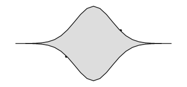
Rendered from the code above.
Drop the kind="mark" and every point that lands near the outline it belongs
to is reported. The exemption needs both sides declared -- a mark near a
tick label really is crowded, and that is most of what the rule is for -- so
the hint tells you which of the two it is:
- "…if
path12is data too, passkind="mark"…" -- the other side is drawn geometry, and declaring it is the fix. - "…so move
tick-label7rather than the mark…" -- the other side is furniture, and the separation really is the fix.
Use kind="mark" only for data-positioned geometry. Applying it to a caption
to suppress a finding leaves the collision unresolved.
Shipping the figure: PDF, and text that cannot be re-shaped
fig.save selects the output format from each suffix. Writing both formats from
one build is useful when the PDF is for publication and the SVG is for editing.
fig = inklet.figure(width="89mm")
sensor = inklet.box("Two-photon\nimaging")
extract = inklet.box("ROI extraction")
fig.add(inklet.vstack([sensor, extract], gap=6))
fig.link(sensor, extract, label="dF/F")

fig.save("figure1.svg", "figure1.pdf")
assert open("figure1.pdf", "rb").read(8) == b"%PDF-1.4"
Figure.to_svg() defaults to live <text> with a font-family chain. The file
is searchable, editable and small, but another machine may resolve the chain
to a different font. Its metrics can differ from those used for layout, causing
labels to overlap box edges without a new Inklet diagnostic.
text="outline" converts glyphs to paths to prevent font substitution:
plain = fig.to_svg()
outlined = fig.to_svg(text="outline")

assert "<text" in plain and "<text" not in outlined
assert "font-family" not in outlined
assert len(outlined) > len(plain)          # glyphs as geometry are not free
In the measured examples below, outlining increases file size by 1.4x to 4x.
Each distinct glyph is defined once in <defs> and reused with <use>.
Outlined text cannot be edited or searched as text. inklet.outline_text(tree)
applies the same conversion to a drawing tree before export.
text="embed" is usually the better trade. Each face is subset down to the
characters this document actually uses and stores inside the file under a name
of its own, so the type is pinned to the exact face it was measured against and
is still live text:
embedded = fig.to_svg(text="embed")

assert "<text" in embedded                 # searchable, selectable, restylable
assert "@font-face" in embedded            # ...and it cannot fall back
assert len(embedded) < len(outlined)
Use either when sharing the file -- a submission, a co-author, a print shop -- and keep the named version alongside for editing. Outline when the destination might not run a modern renderer at all; embed otherwise.
Whichever you pick, the type arrives as the type you measured. A block is
outlined under the OpenType features it was shaped with -- they travel on
the prim, so there is no parameter to pass and none to get wrong -- and a run
recoloured by {fill|text} keeps its colour through all three spellings:
keyed = inklet.text("the {accent|measured} curve and the {#c1121f|fit}")
for document in (inklet.to_svg(keyed),
                 inklet.to_svg(keyed, text="outline"),
                 inklet.to_svg(inklet.outline_text(keyed))):
    assert "#0072b2" in document and "#c1121f" in document

digits = inklet.text("0123456789", features={"tnum": True})
assert digits.prim.features == (("tnum", True),)
PDF outlines by default, for the same reason: it is the shipping format, and a
PDF that depends on a font being installed is not one. That is also why the PDF
is often smaller than the SVG it came from -- the content stream is deflated,
which more than pays for the outlines on anything with a mesh in it.
fig.to_pdf(text="embed") makes it searchable instead; the recipe at the end
of this file measures both.
A label that clears its target
A callout is three decisions -- where the text goes, how far off the shape it
sits, and where the leader touches -- and hand-placing it means redoing all
three every time the shape moves. inklet.annotate makes them one call. The
clearance is measured against the target's silhouette, not its bounding box,
so a label on the north-east of a round cell sits 2.5mm off the curve rather
than 2.5mm off an empty corner.
soma = inklet.circle(width=16, height=11, fill=TH.color(0), stroke="none")
callout = inklet.annotate(soma, "layer 5 pyramidal", side="ne", clear=2.5)

assert inklet.annotation_side(callout) == "ne"
The leader is a real link(kind="leader"), so it stops on the shape's boundary
at one end and short of the type at the other. annotate returns a Diagram
with the target inside it, which is what makes it chain: annotate the result to
hang a second label on a second part, and every label already placed becomes an
obstacle the next one avoids.
steps = inklet.vstack([inklet.box("wash"), inklet.box("stain"), inklet.box("image")], gap=4)
wash, stain, image = steps.children

scene = inklet.annotate(wash, "PBS, 3x", side="e", within=steps)
scene = inklet.annotate(stain, "anti-GFP, overnight", side="e", within=scene)
scene = inklet.annotate(image, "20x, 3 fields", side="e", within=scene)

protocol = inklet.figure(width="89mm")
protocol.add(scene)
assert protocol.lint() == []
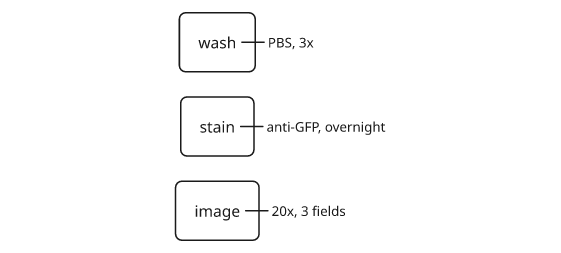
Rendered from the code above.
within= is how the second call is told which drawing to measure in: the
target is buried in a tree by then, and a label placed against the box's own
frame would ignore everything around it.
When the requested side is occupied, annotate walks outward around the
compass -- n, then ne, nw, e, w -- and takes the first side that is
clear. Pass the things it must not cover as avoid=, and read back where it
ended up:
core = inklet.box("reactor")
key = inklet.box("legend").translated(0, -9)      # y grows downward: due north
picture = inklet.place([core, key])

moved = inklet.annotate(core, "80 degC", side="n", avoid=[key], within=picture)
assert inklet.annotation_side(moved) == "e"
The order is fixed, so the same figure gives the same answer every run.
inklet.annotation_side reports when the selected side differs from the request.
Insets and brackets
An inset is useful when a reader can identify which part of the picture got
bigger. Panel.inset puts a second panel in a corner on a plate, and
zoom= in the parent's data coordinates draws the window it magnifies and
joins the two with connectors that stay outside both rectangles.
decay = [(t, 100 * 2.718 ** (-t / 9)) for t in range(25)]

main = inklet.panel(72, 44, x=(0, 24), y=(0, 100))
main.line(decay)
main.axes(x="bottom", y="left")

early = inklet.panel(26, 16, x=(0, 4), y=(60, 100))
early.line(decay[:5])
early.outline()

main.inset(early, corner="ne", zoom=(0, 4, 60, 100))
main.bracket(6, 12, 70, text="***")

plot = inklet.figure(width="89mm")
plot.add(main.build())
assert plot.lint() == []
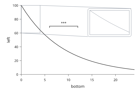
Rendered from the code above.
The inset is scaled to width= as a fraction of the plot area -- 0.35 by
default -- including its text. A third-size inset has third-size tick labels,
and inklet.lint reports them at 5pt. Build the subpanel near its finished size
and pass width=None to preserve its dimensions and typography.
Panel.bracket(x0, x1, y, text=...) takes data for the span and millimetres
for the tick length, because a tick is a mark on the page and has no meaning in
the data. Off a panel, inklet.bracket(a, b, side="n", text="***") does the same
between two points or two diagrams, and inklet.dimension(a, b, "12.4 mm") is its
engineering cousin -- witness lines, end ticks, a label on a plate over the
line.
Panel letters
Every multi-panel figure may need panel letters. Placing them at the panels'
bounding-box corners puts them inside
the y-axis labels, because the axis is part of the panel. inklet.letters places
them outside and returns tagged diagrams in the given order, so the handles
you already have keep working.
left = inklet.panel(40, 30, x=(0, 1), y=(0, 1))
left.outline()
left.axes(x="bottom", y="left")

right = inklet.panel(40, 30, x=(0, 1), y=(0, 1))
right.outline()
right.axes(x="bottom", y="left")

tagged = inklet.letters([left, right])
sheet = inklet.figure(width="178mm")
sheet.add(inklet.hstack(tagged, gap=8))
assert sheet.lint() == []
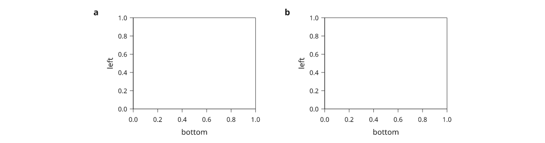
Rendered from the code above.
start="c" continues a sequence across a figure built in pieces, and
style="paren" or "upper" matches the journal. The letters are kind="title"
so they take the theme's panel-title role -- bold, one size up -- rather than
needing a style override to look like everybody else's.
Bars, errors and a histogram
A bar chart is not a special kind of figure, it is a panel with rectangles in
it, so it is built the same way as everything else: a Band scale across the
categories, bars for the rectangles, errorbars over them. Both take data
coordinates -- the category name on a band axis, the value on the other -- and
neither needs the author to convert anything to millimetres.
import math

GROUPS = ["ctrl", "low", "mid", "high"]
MEAN = [12.1, 24.8, 31.4, 18.2]
SEM = [1.2, 2.0, 1.6, 2.4]

bars = inklet.panel(44, 32, x=GROUPS, y=(0, 40))
bars.bars(GROUPS, MEAN)
bars.errorbars(list(zip(GROUPS, MEAN)), yerr=SEM)
bars.axes(y="response / AU")

N = 400
SAMPLE = [math.sqrt(-2 * math.log((i + 0.5) / N))
          * math.cos(2 * math.pi * (i * 0.618034 % 1.0)) for i in range(N)]
edges, counts = inklet.histogram(SAMPLE, 12)

spread = inklet.panel(44, 32, x=(edges[0], edges[-1]), y=(0, max(counts)))
spread.hist(SAMPLE, 12)
spread.axes(x="z score", y="count")

sheet = inklet.figure(width="120mm")
sheet.add(inklet.hstack([bars.build(), spread.build()], gap=10, align="top"))
assert sheet.lint() == []
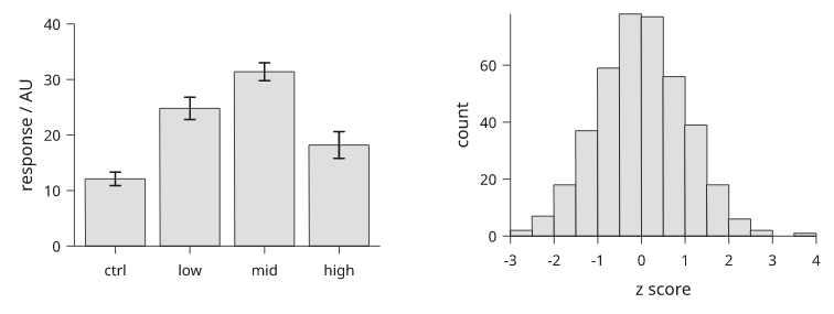
Rendered from the code above.
A single bar series defaults to a grey fill with a dark outline. Pass bars
a list of lists to draw multiple series using the palette, grouped side by side
unless stacked=True is supplied.
inklet.histogram is separated from Panel.hist on purpose: you need the counts
before you can build the y scale, and the bin edges before you can build the x
one. It quantises the edges onto the same 1/2/5 lattice the ticks use, so the
bins fall on numbers a reader can read -- -3.0 to 4.0 in steps of 0.5
here, not twelve equal slices of whatever the extremes happened to be. Pass a
list of edges instead of a count to place them yourself, and density=True to
divide by the sample size and the bin width so two samples of different sizes
can be compared.
errorbars takes one number, one number per point, or a (low, high) pair per
point for an asymmetric interval; xerr= does the same across. stroke= (or
color=) is one colour for every whisker, or one colour per point.
A twin y axis
Two quantities against one x -- a current in mA and an efficiency in percent --
are two scales over one rectangle. Panel.twin_y gives you the second scale
and returns a panel handle: everything you draw
on it lands in the same picture, mapped through the second scale.
TH = inklet.current_theme()
TIME = list(range(0, 25, 2))
CURRENT = [0.0, 4.2, 7.8, 10.1, 11.6, 12.4, 12.9,
           13.1, 13.2, 13.3, 13.3, 13.4, 13.4]
EFFICIENCY = [0, 62, 74, 80, 83, 85, 86, 86, 87, 87, 88, 88, 88]

cell = inklet.panel(64, 40, x=(0, 24), y=(0, 15))
cell.line(list(zip(TIME, CURRENT)))
cell.axis("bottom", label="time / h")
cell.axis("left", label="current / mA")

eff = cell.twin_y((0, 100), label="Faradaic efficiency / %", color=TH.color(5))
eff.line(list(zip(TIME, EFFICIENCY)), stroke=TH.color(5), stroke_dash=(1.2, 0.8))
eff.scatter(list(zip(TIME, EFFICIENCY)), color=TH.color(5))

cellfig = inklet.figure(width="89mm")
cellfig.add(cell.build())
assert cellfig.lint() == []
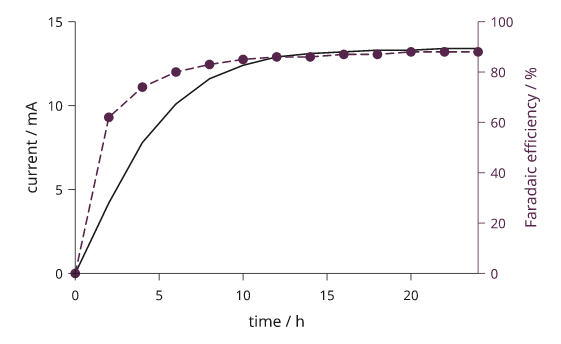
Rendered from the code above.
Build the panel on which you called twin_y, rather than the returned twin:
the twin uses its parent's content. color= sets the second axis's spine,
ticks and numbers. Match it to the associated series and identify the mapping
in the legend or caption. Choose a colour with sufficient text contrast;
inklet.lint checks tick labels, and the paler palette colours do not meet
4.5:1 contrast against white.
twin_x is the same thing across the top -- wavelength above frequency, or a
second time base.
Facets that share axes
Several panels of the same plot need one set of axes between them, not one set
each. inklet.facets lays them out on a grid, aligns them on their plot areas
rather than on their bounding boxes, and writes the numbers only where a reader
would look for them: under the bottom panel of each column, left of the first
of each row.
DOSES = [0, 1, 3, 10]
ANIMALS = {
    "m1": [2.0, 5.1, 8.9, 12.2],
    "m2": [1.6, 4.4, 8.1, 11.0],
    "m3": [2.4, 5.8, 9.6, 13.1],
    "m4": [1.9, 4.9, 8.6, 11.8],
}

cells = []
for name, values in ANIMALS.items():
    q = inklet.panel(34, 22, x=(0, 11), y=(0, 14))
    q.line(list(zip(DOSES, values)))
    q.scatter(list(zip(DOSES, values)))
    q.title(name)
    cells.append(q)

gridfig = inklet.figure(width="89mm")
gridfig.add(inklet.facets(cells, cols=2, count=4,
                       x_label="dose / mg kg^{-1}",
                       y_label="AUC / h ng mL^{-1}"))
assert gridfig.lint() == []
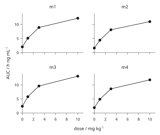
Rendered from the code above.
Every panel keeps its spine and its ticks; only the repeated numbers go, so an inner panel is still a plot with a scale on it. The shared names are centred on the block of plot areas, not on the grid's bounding box -- centring on the box puts the name visibly left of the data, because the first column's numbers stick out and nothing balances them on the right.
Anything facets does not recognise is passed to every axis it builds, so
count=4, minor=True, si=True or format=" %" style the whole grid at
once. axes=False leaves the furniture to you and does the alignment only,
which is what you want when the panels already include their own axes.
Keep the file small, or keep it readable
Path data is most of an SVG that has any real geometry in it -- 88% of the
bytes on a shaded 3D panel. to_svg writes it two ways, and picks per path.
The default, compact="auto", spells short paths out (M 12.5 -3 L 14 -3 Z)
so a frame or a callout leader can still be hand-edited, and packs anything
over 32 commands into the relative, elided form (m12.5-3h1.5z) that no one
reads anyway.
import math

wave = inklet.panel(70, 34, x=(0, 12), y=(-1.1, 1.1))
wave.line([(x / 40, math.sin(x / 6)) for x in range(481)])

small = inklet.figure(width="89mm")
small.add(wave.build())

packed = small.to_svg()                   # the default: long paths packed
spelled = small.to_svg(compact=False)     # every coordinate from the origin
assert len(packed) < 0.75 * len(spelled)
assert small.to_svg() == packed           # and byte-identical on a re-render
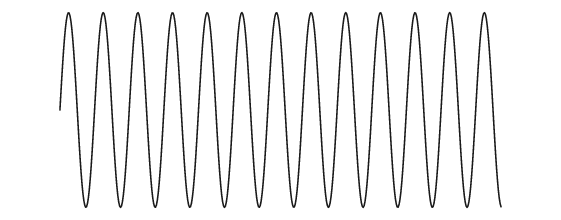
Rendered from the code above.
compact=True packs every path, however short; compact=False packs none.
Use False when someone will edit the
geometry by hand, or when you need the coordinates to be absolute: a
renderer accumulates relative steps in single precision, which moves
antialiased edges by a fraction of a device pixel. The difference is usually not
visible, but the option is explicit for workflows that require absolute
coordinates.
The other setting that changes file size is text handling. Measured on
the corpus, as a multiple of the default text="names" file:
| figure | names | text="embed" |
text="outline" |
|---|---|---|---|
hello_figure |
5.5 kB | 1.80x | 4.15x |
panels |
55 kB | 1.15x | 1.60x |
hard_figure |
45 kB | 1.26x | 2.72x |
mega_figure |
908 kB | 1.06x | 1.39x |
Embedding has a smaller proportional cost in geometry-heavy figures because
each font subset is stored once. Outlining adds glyph paths and removes the
need for the destination renderer to load fonts. Both use the face selected
during layout. Gzip reduces all three files: in the recorded hard_figure
comparison, compressed sizes are 6.5 kB with named fonts, 14 kB embedded and
26 kB outlined.
Placing solids in a scene
An assembly is a inklet.scene: several meshes, one camera, one scale. Where each
part stands is said in its own options -- at= is the point its origin lands
on, spin= is (axis, degrees) or three Euler angles, scale= is one number
or three. They apply in that order, scale then spin then move, which is the
only order in which the numbers mean what they look like: scale= is about the
solid's own centre, and at= is a place rather than a displacement some later
rotation swings elsewhere. The same three work on inklet.solid() and
inklet.model().
from inklet.three import build

plate = build("box", size_x=0.25, size_y=4.0, size_z=4.0)
rod = build("cylinder", radius=0.12, height=5.0, segments=20)

rig = inklet.scene([
    ("far", plate, {"at": (-0.9, 0, 0)}),
    ("near", plate, {"at": (0.9, 0, 0)}),
    ("rod", rod, {"spin": ("y", 90)}),
], width=64, view="three-quarter", style="shaded",
    assert_order=[("near", "far")])

fig = inklet.figure(width="89mm")
fig.add(rig)
assert fig.lint(rules=["DEPTH_ORDER"]) == []
assert_order=[("near", "far")] is the recipe's real subject. It says the
first part has to come out in front of the second, and inklet.lint checks that
against the projected geometry rather than against the code -- so the claim
survives the camera being turned, a part being added between the two, or the
numbers coming from data next time. It reports an error three ways: the parts
are painted the other way round, they do not overlap on the page at all, or
they overlap and the claim is simply false.
Every part also answers to its own projected box, so a leader has somewhere to
aim without any arithmetic. rig.at("rod") is the part's centre,
rig.at("near.nw") and its seven companions are the compass points around it,
and a 3D point a part names for itself ({"anchors": {"tip": (2.5, 0, 0)}})
comes along under the same prefix.
tag = inklet.label("tie rod")
sheet = inklet.figure(width="89mm")
sheet.add(inklet.hstack([tag, rig], gap=8.0, align="center"))
sheet.link(tag, rig.at("rod"), kind="leader", through=(rig,))

plates = inklet.three.parts_of(rig, lambda part: part.name != "rod")
assert [part.name for part in plates] == ["far", "near"]
assert sheet.lint(rules=["LINK_CROSSES"]) == []
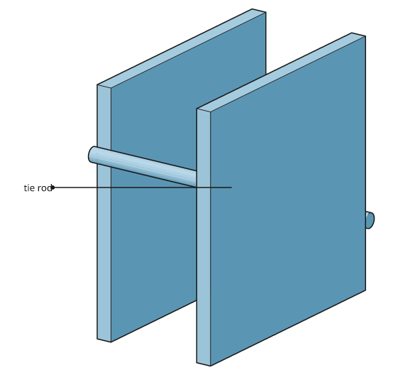
Rendered from the code above.
through=(rig,) is the other half. A leader aimed into an assembly usually has
to cross something on its way in -- a cage rod, an outer plate -- and that is
not a mistake; citing the whole scene exempts every part inside it, because the
rule asks whether the crossed node is inside anything the link declared.
inklet.three.parts_of(rig, ...) narrows that to some of the parts, which is what
you want when the arrow still has to be checked against the one it stops on.
Parts are painted furthest centre first, which is right until a part's centre
is not where its geometry is -- a nut standing proud of a plate, a rod through
nine of them. DEPTH_ORDER finds those too, without being asked. Its two
answers are order="exact", which settles depth facet by facet across the
whole scene, and saying the order yourself with behind=, in_front_of= or
draw_order= on the part; the rule takes any of the three as the answer and
stops second-guessing that part.
order="exact" draws the assembly in one pass, so a part can no longer set its
own style or opacity -- those belong to a pass, and there is one. What it
can still set is color, colors and stroke_width, the three the fused
mesh stores per face group. Line weight identifies parts in a technical
illustration:
threaded = inklet.scene([
    ("ring", build("torus", radius=0.5, tube=0.12, segments=32, rings=14)),
    ("rod", build("cylinder", radius=0.1, height=2.0, segments=24),
     {"stroke_width": 0.6}),
], width=50, view="three-quarter", style="shaded", order="exact")

assert inklet.lint(threaded) == []
A plate with a hole
Drawing a bolt hole as a disc on the front face works until the camera moves:
there is nothing behind the disc, so the far wall of the plate shows through
it, and hidden-line removal has no wall to hide anything behind. Mesh.drill
cuts the geometry instead. The result is still closed -- every edge shared by
exactly two faces -- which is what keeps silhouettes, shading and the exact
sort working on it.
from inklet.three import build

plate = build("box", size_x=4.0, size_y=3.0, size_z=0.4)
for x, y in ((-1.4, -0.9), (1.4, -0.9), (1.4, 0.9), (-1.4, 0.9)):
    plate = plate.drill("z", radius=0.3, at=(x, y, 0), group="hole")

assert plate.is_closed

drilled = inklet.model(plate, width=60, view="three-quarter", style="shaded",
                    colors={"hole": TH.muted})

sheet = inklet.figure(width="89mm")
sheet.add(drilled)
assert sheet.lint(rules=["OFF_CANVAS"]) == []
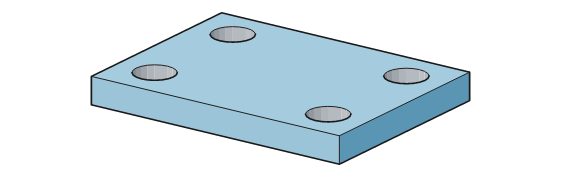
Rendered from the code above.
axis= defaults to "z" and takes "x", "-y", or a vector; at= is a point
in the mesh's own frame that the axis passes through; group= names the wall
faces, so colors= can darken the bore. segments= sets the number of sides.
Small holes may need fewer facets: choose a count that preserves the outline at
print size while limiting the geometry that must be depth-sorted and exported.
This plate is what the default sort is for. sort="auto" settles a mesh of
up to 2000 faces pairwise -- facet against facet -- rather than by each facet's
mean depth, and a drilled plate is the shape that needs it: the wall of a bore
is a ring of small facets ranked against one large side face whose centre is
nowhere near where the bore meets it. Ask for sort="depth" here and the hole
nearest the front edge comes out with its wall painted over the side of the
plate. Every hole is drawn, three of the four are right, and the fourth is the
one a reader notices. It is the same failure DEPTH_ORDER reports between the
parts of a scene, one level down. Above 2000 faces auto goes back to the
centres, because the pairwise test is quadratic grid work and a 60k-face
protein has to be drawn in a second, not a minute; sort="exact" asks for it
at any size and sort="depth" declines it at any size.
A hole through a flat face is cut a face at a time, re-triangulating the whole face and adding no points to its border -- which is what keeps the mesh watertight where the untouched side walls meet it. A hole through a curved wall cannot be done that way, because the facets it comes out through are in different planes, so those are cut one facet at a time and welded. Both come out closed:
pipe = build("cylinder", radius=1.0, height=3.0, segments=32)
pipe = pipe.drill("x", radius=0.3, segments=20, group="port")
assert pipe.is_closed
inklet.solid("tube", radius=, bore=, height=) is the shortcut for the commonest
version of that -- a cylinder bored along its own axis. Prefer it to drilling a
cylinder: the bore gets its own segments, so the hole is as round as the
outside, and the ends come out as two annular rings rather than as the fan of
triangles a re-triangulated cap leaves behind.
port = inklet.solid("tube", width=40, view="three-quarter", style="shaded",
                 radius=0.42, bore=0.3, height=1.6)
assert inklet.lint(port) == []
What is still refused, by name rather than as a mesh with a gap in it: a hole
that runs off the edge of the part or into another hole, one that does not go
in one side and out another, and one whose circle grazes a corner of the
surface it comes out through -- which a small nudge to at= or radius=
moves off. For anything genuinely boolean, Mesh.subtract(tool) uses trimesh
when it is installed.
Three tones, and which line is heaviest
style="shaded" uses the theme's stroke width for silhouettes, 0.62 of that
width for creases, and no line at tone boundaries. This distinguishes the outer
shape from surface folds without outlining each shading band. Stroke widths
remain physical: a 0.25 mm line stays 0.25 mm whether the solid is 18 mm or
80 mm wide.
style="toon" is the same drawing with the shading turned into three flat
bands instead of twenty steps, cut smoothly so the boundaries are the isolines
they stand for rather than the staircase of whichever facets tipped across the
step. It is "shaded" plus four numbers, all still overridable:
import inklet.three

assert dict(inklet.three.TOON) == {"shading": "smooth", "levels": 3,
                                "lift": 0.55, "shade": 0.42}

cartoon = inklet.solid("torus", width=40, view="three-quarter", style="toon")
counted = inklet.solid("torus", width=40, view="three-quarter", style="toon",
                    levels=6)
assert inklet.lint(cartoon) == [] and inklet.lint(counted) == []
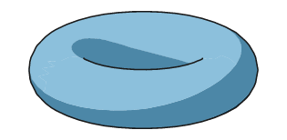
Rendered from the code above.
shading="smooth" applies smooth surface shading. Flat shading gives a facet
one tone, so a band boundary follows facet edges and staircases;
the auto-tessellation picks segment counts from the outline's chord error,
which at 54 mm leaves facets several millimetres across -- invisible on the
silhouette, very visible in the tone. It produces about 40% more path data on a
sphere. Use it for coarse curved bodies; on fine meshes the additional detail
may not be perceptible.
A key that cannot describe a picture that is not there
Writing a legend out by hand is how a figure ends up naming a series it no
longer draws, or naming it in a colour it was never drawn in. KEY_MISMATCH
catches the worst of that after the fact; naming the series at the point you
draw it means there is nothing to catch. Every drawing call takes name=, the
panel remembers what that name was actually drawn as -- colour, dash, marker,
fill -- and legend() builds the block from the record.
import math

T = [i / 4.0 for i in range(41)]
DECAY = [math.exp(-t / 3.0) for t in T]
SPREAD = [0.02 + 0.03 * t for t in T]

sig = inklet.panel(60, 34, x=(0, 10), y=(0, 1.1))
sig.band(T, [max(0.0, m - s) for m, s in zip(DECAY, SPREAD)],
         [m + s for m, s in zip(DECAY, SPREAD)], name="model")
sig.line(list(zip(T, DECAY)), name="model")
sig.scatter([(t, math.exp(-t / 3.0) + 0.04 * math.cos(t * 5))
             for t in T[2:-2:4]], name="observed")
sig.axes(x="t / h", y="signal").legend(corner="ne")

assert [e.name for e in sig.keys] == ["model", "observed"]
assert inklet.lint(sig.build()) == []
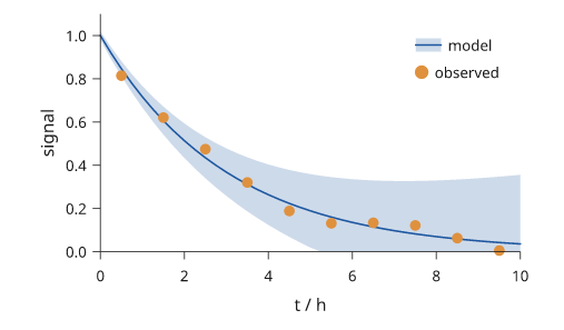
Rendered from the code above.
Three things fall out of the record that are tedious to keep true by hand.
One name, one entry. The band and the line share the name "model", so
they are one row, and the swatch shows both: a line over its own tint. Draw the
band without a colour and it takes the line's, whichever order the two calls
came in.
Colours assign themselves. A named series with no stroke= takes the next
palette colour, counted over the names rather than over the calls -- so the
band does not spend a colour. Pass stroke= and it is never overridden.
p.keys is readable before the legend exists, which is what lets you assert
on it, or lay the key out yourself with entries= while still reading the
colours off the panel.
legend(corner=...) puts the block inside the plot area, legend(side=...)
stands it outside; columns= matters more than it sounds on an 89mm column,
where three entries stacked vertically is most of a panel's height.
The one thing to watch is above: band is not clipped to the domain, because
nothing in inklet.plot is -- data that leaves the panel draws where the data
says. Here the lower edge would go below zero at large t and paint over the
tick labels, and the linter reports the overlap. max(0.0, ...) says what you
mean, which is that the interval is bounded below.
A matrix too big to draw one rectangle at a time
Panel.matrix draws a rectangle per cell, which is right for a 12 x 30 array
and wrong for a 90 x 120 one: 10,800 nodes is about a megabyte of SVG that no
editor will open happily. Above a few thousand cells the panel builds a PNG
instead, at exactly one pixel per cell, and hands the renderer an image with
smoothing turned off. Nothing about the call changes.
BIG = [[math.sin(r / 9.0) * math.cos(c / 6.0) for c in range(120)]
       for r in range(90)]
shades = inklet.ramp("tol-sunset")
field_scale = inklet.linear((-1.0, 1.0))

heat = inklet.panel(52, 39, x=(0, 119), y=(0, 89))
heat.matrix(BIG, ramp=shades, scale=field_scale)
heat.axes(x="x / um", y="y / um").colorbar(label="dF/F")

fig = inklet.figure(width="90mm", theme="nature")
fig.add(heat.build())
assert len(fig.to_svg()) < 60_000
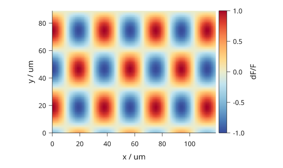
Rendered from the code above.
raster="auto" is the default: vector below the threshold, pixels above it.
raster=True forces it and is useful for a matrix you know is going into a
figure with twenty others -- and raster=False keeps rectangles no matter how
many there are, which is what you want if the cells must be individually
selectable in Illustrator.
One pixel per cell, never resampled. The image is the size of the array,
not the size of the panel, and it is scaled up by the viewer with
image-rendering: pixelated. A cell edge lands where the rectangle's edge
landed, so a raster matrix and a vector one are the same picture; the tests
assert that by drawing both and comparing. The consequence is that the file
does not grow when the panel does -- a 90 x 120 field is about 3kB whether it
is printed at 40mm or 180mm.
It is a picture of the data, so the data has to be there. A NaN cell is
refused by name rather than painted as whatever the ramp returns for a
non-number, and cells that are not evenly spaced cannot be pixels at all --
pass x=/y= edges that step unevenly and raster=True is an error. With
raster="auto", unevenly spaced cells remain vector even when the cell-count
threshold is exceeded.
colorbar() takes its ramp and its scale from the matrix that was drawn, so
the key and the picture cannot disagree even when the raster path has thrown
the rectangles away.
An axis of dates
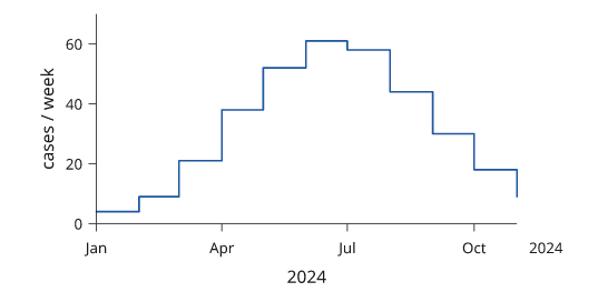
Give a panel two dates and it reads them: x=("2024-01-01", "2024-12-31") is a
time scale, not two strings and not two numbers. ISO 8601 text,
datetime.date and datetime.datetime are all accepted and all mean one
instant; a tzinfo is dropped, because a figure is a picture of one clock.
DAYS = [f"2024-{1 + n // 30:02d}-{1 + n % 30:02d}" for n in range(0, 330, 30)]
LEVEL = [4, 9, 21, 38, 52, 61, 58, 44, 30, 18, 9]

epi = inklet.panel(60, 30, x=(DAYS[0], DAYS[-1]), y=(0, 70))
epi.step(list(zip(DAYS, LEVEL)), name="cases")
epi.axes(x="2024", y="cases / week")
assert inklet.lint(epi.build()) == []
Rendered from the code above.
The ticks walk the calendar rather than adding a constant, which is the whole
reason this is not a linear with a formatter: months are not 30 days, and an
axis that ticks every 30.44 days puts a label three days into February. Ticks
land on round units -- New Year, the first of the month, midnight, the hour --
and the label is written at the coarseness of the ticks that were actually
chosen: years, months, days or clock times.
The year is written on the first tick, and again wherever it changes. A
twelve-month axis inside 2024 is labelled Mar 2024 Apr May ..., so the year
is never left detached past the last tick. Straddle New Year and each January
gains its year: Oct 2023 Nov Dec Jan 2024. A clock axis does the same with the
date, which is written on the first tick and at each midnight: 3 May 2021 00:00
06:00 12:00 18:00.
inklet.dates(domain, range) builds the scale directly when you want to share it
between panels, and minor=True on the axis divides into the next unit down --
months inside years, days inside months -- dropping them all when they would
not clear each other.
Writing on the plot, in the plot's own units
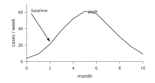
After drawing data, authors commonly add a word beside a point, an arrow between positions, or a caption on a peak. Plotting methods accept data coordinates for these additions and perform the mapping to millimetres.
PEAK = max(range(len(LEVEL)), key=LEVEL.__getitem__)

note = inklet.panel(60, 30, x=(0, 10), y=(0, 70))
note.line(list(zip(range(11), LEVEL)))
note.annotate(PEAK, LEVEL[PEAK], "peak", side="n")
note.text(0.4, 62, "baseline", anchor="w", size=TH.font_size_small)
note.arrow((0.4, 58), (2.0, 24))
note.axes(x="month", y="cases / week")
assert inklet.lint(note.build()) == []
Rendered from the code above.
text(x, y, ...) puts a label on a data point; anchor= is a compass point on
the label, so anchor="w" sets its west edge on the datum and the writing
runs east from there. offset= nudges it afterwards in millimetres, which is
the right unit for a nudge: it is a typographic clearance, not a quantity.
arrow(a, b) runs between two data points through inklet.links, so the head is
the head every other arrow in the figure has, and both ends are anchors rather
than shapes -- the arrow ends on the coordinates exactly, with nothing clipped
back.
annotate(x, y, text) searches for a label position beside the datum and adds
a leader to it. side= requests a starting side; when blocked, the search tries
other directions. inklet.annotation_side reports the chosen side.
Labels stay inside the plot area by default, even when the datum lies just
outside the axis range: the label slides in rather than hang over the edge.
Pass inside=False to allow outside placement. color= sets the words and the
leader together. avoid=[...] supplies rectangles the label must avoid,
for example a legend's bounds.
front=False on any of the three puts the writing under the data instead of
over it.
Waypoints, trunks and loops
Four connector shapes that are not one line between two boxes. All four are
keywords on fig.link, and inklet.graph passes anything it does not recognise
in an edge mapping straight through to it.
A route you chose yourself. waypoints= is points the line must visit, in
order, in figure coordinates -- Vec2, an (x, y) pair, or shape.at("n") to
hang the detour off something that moves. A straight route joins them with a
polyline, an orthogonal one takes Manhattan legs between them, and avoid
searches between consecutive waypoints rather than over the whole page. That
last one is the cheap way to tell the router the one thing it cannot work out
for itself and get exactly the corridor back.
left, right = inklet.box("read"), inklet.box("write")
row = inklet.hstack([left, right], gap=40)
fig = inklet.figure(width=90)
fig.add(row)
fig.link(left, right, route="orthogonal",
         waypoints=[(0, -14)], label="retry")
assert fig.lint() == []
The label, the arrowhead and LINK_CROSSES all read the polyline that was
actually drawn, so a detour is not something the rest of the library has to be
told about separately.
One stem, one fork. A list on either side of a link is a trunk:
fig.link(a, [b, c, d]) leaves a once and divides, and fig.link([a, b], c)
is the merge. route="orthogonal" draws it as a bus -- stem, rail, a drop into
each shape -- and anything else draws it as a fan out of one fork point.
stem= is how far along the stem the fork happens.
source = inklet.box("parse")
sinks = [inklet.box(t) for t in ("html", "pdf", "text")]
tree = inklet.hstack([source, inklet.vstack(sinks, gap=4)], gap=24)
fig = inklet.figure(width=90)
fig.add(tree)
fig.link(source, sinks, route="orthogonal")
assert fig.lint() == []
Three separate links out of parse would draw three lines over the same
first centimetre and earn a COINCIDENT_SHAFT. A trunk is one stroke, so
there is nothing there to report -- and the reader can see it is one signal.
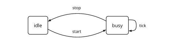
A loop, and a pair that argue. fig.link(a, a) is a self-loop; loop=
names the side ("n", "e", "s", "w") and leaving it out picks the side
with the least ink on it. offset= bows a link off the straight line by that
many millimetres, positive to the right of travel, so two arrows between the
same pair given the same offset come out on opposite sides with a label
each.
a, b = inklet.box("idle"), inklet.box("busy")
pair = inklet.hstack([a, b], gap=30)
fig = inklet.figure(width=90)
fig.add(pair)
fig.link(a, b, offset=4, label="start")
fig.link(b, a, offset=4, label="stop")
fig.link(b, b, loop="e", label="tick")
assert fig.lint() == []
Rendered from the code above.
The automatic side is decided against every other shaft on the page, and against the plate every other label reserves, not just the ones declared before it. Name the side anyway when two sides are equally clear and you have a preference: the tie is broken by compass order, not by taste.
Three arrows out of one face. port= slides an end along the face it
leaves through, and target_port= does the same at the other end. inklet.graph
already spreads its own ports; this is for links you place by hand.
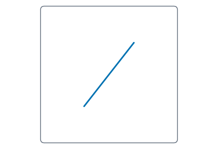
An anchor that survives being turned
d.rotated(30) wraps d in a new parent and preserves its identity, so links
to d still resolve after further layout. Registered anchors also resolve
through wrappers before and after layout; callers can use them without
retaining a separate reference to the original node.
import math

arm = inklet.polyline([(0, 0), (26, 0)], stroke=TH.accent, stroke_width=TH.thick)
arm.anchor("tip", (1.0, 0.5))          # right edge, half way down
turned = arm.rotated(-52)

# `anchor_point` is local -- before the node's *own* transform -- so the turn
# shows one frame out, wherever the turned arm has been put.
tip = turned.translated(0, 6).anchor_point("tip")
assert round(tip.x, 6) == round(13 * math.cos(math.radians(-52)), 6)
assert round(tip.y, 6) == round(13 * math.sin(math.radians(-52)), 6)

fig = inklet.figure(width=70)
fig.add(inklet.overlay([inklet.box(width=44, height=44, stroke=TH.muted), turned]))
tree, places = fig.build()
here = places[turned.id]
assert round((here.point("tip") - here.point("center")).length, 6) == 13.0
assert fig.lint() == []
Rendered from the code above.
Two things it deliberately will not do. A compass name is not a point of a
shape but a side of a box, so it is always answered from the node you asked --
a child that registered an anchor called "e" cannot shadow the wrapper's
east. And only a transform wrapper answers for its child, never a group: an
hstack of five drawn shapes has five origin anchors and no shared one, so
asking the stack for "origin" still raises rather than handing back the first
one it finds.
Putting one drawn shape back where it was drawn. inklet.drawn([...])
composes several shapes on the frame they share; inklet.as_drawn(shape) is the
one-shape form, for when you are assembling the container yourself -- another
Panel.over list, a scene you are building child by child.
tail = inklet.polyline([(12, -5), (20, -9), (34, -10)], stroke=TH.color(1))
assert inklet.as_drawn(tail).bbox == inklet.Rect(12.0, -10.0, 34.0, -5.0)
It asks the node it was handed, not through it: a wrapper you put round a drawn
shape is a placement you meant, and as_drawn will not undo it.
One part of a scene, drawn on top of it
order="exact" provides exact depth by fusing the parts into one mesh. A part
then stops being an independent rendering unit: one hidden-line pass and one
facet sort for the whole scene, so only properties stored per face
group -- color, colors, stroke_width -- may still differ between parts. A
part asking for style="lineart" inside a shaded scene is refused rather than
ignored because there is no separate pass for it.
overlay=True renders a part separately. The part is left out of the fused mesh and drawn
as its own model() in the scene's own projection, so it takes everything
model() takes -- style, opacity, hidden, cull, occlusion, sort.
from inklet.three import build

frame = build("box", size_x=4.0, size_y=0.5, size_z=2.4)
shaft = build("cylinder", radius=0.35, height=5.0, segments=20)
case = build("box", size_x=5.4, size_y=2.6, size_z=3.4)

rig = inklet.scene([
    ("frame", frame),
    ("shaft", shaft, {"spin": ("y", 90)}),
    ("case", case, {"overlay": True, "style": "lineart", "cull": False,
                    "opacity": 0.45}),
], width=70, view="three-quarter", style="shaded", order="exact")

fig = inklet.figure(width="89mm")
fig.add(rig)
assert rig.at("case.ne") is not None
assert fig.lint(rules=["DEPTH_ORDER"]) == []
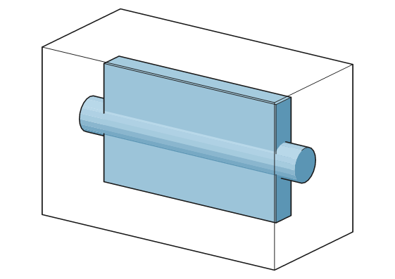
Rendered from the code above.
An overlay is drawn above the depth-sorted scene and can cover underlying content. Use it for a translucent enclosure, a cutting plane or a line-art part over a shaded assembly. Keep a part in the fused mesh when it must participate in depth sorting with the rest of the scene.
Two overlays are drawn in their declared order. DEPTH_ORDER treats an overlay
as an explicit ordering choice, as it does draw_order=, and does not report
that choice as a depth-order error.
An overlay is still a part in every other way: it keeps its name, its anchors,
its silhouette for an arrow to clip on, and its entry in inklet.three.parts_of.
overlay=True under order="parts" is an error, because there every part is
already its own node with its own style; so is a scene in which every part is
an overlay, which is order="parts" written the long way.
When to cut the data at the plot edge
inklet.plot does not clip by default. A trace that leaves the panel remains in
the data, and the linter reports a mark outside the plot area. This preserves
the distinction between an out-of-domain value and a clipped display.
Sometimes you did. A long recording shown at the range the reader cares about,
a density whose kernel tail runs past the axis, a scatter with three points at
infinity: clip those, and say so in the caption. clip=True on the panel
clips everything drawn in it; clip= on one call decides that call.
import inklet

TH = inklet.use_theme("nature")
RAW = [(t / 4.0, (1.0 if t % 37 else 6.0) * (1 + 0.2 * (t % 5))) for t in range(200)]

trace = inklet.panel(60, 30, x=(0, 50), y=(0, 3), clip=True)
trace.line(RAW, name="raw")
trace.hline(2.0, label="threshold", stroke_dash=(1.0, 0.8))
trace.axes(x="t / s", y="dF/F")

fig = inklet.figure(width="89mm")
fig.add(trace.build())

# The clip is geometric rather than an SVG clipPath, so the envelope -- and
# so the linter, and so any figure this panel is stacked into -- sees the cut
# shape and not the data's own extent.
loose = inklet.panel(60, 30, x=(0, 50), y=(0, 3))
loose.line(RAW, name="raw")
loose.hline(2.0, label="threshold", stroke_dash=(1.0, 0.8))
loose.axes(x="t / s", y="dF/F")
assert trace.build().bbox.height < loose.build().bbox.height
Two things are never clipped, because a half of either is worse than none:
words, and anything you drew with text, annotate, bracket or a labelled
rule. p.line(..., clip=False) puts one series back outside the box on an
otherwise clipped panel.
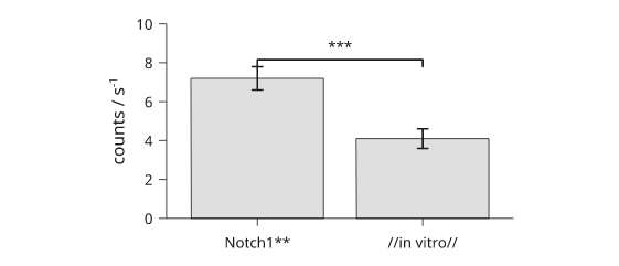
Data strings are read literally, which matters the day a category is called
Notch1** or //in vitro//: categories, series names and legend names go to
the page as written. Prose -- axis names, titles, p.text -- is markup, so
x="v / mm s^{-1}" still lifts its exponent, and p.text(..., markup=False)
opts one string back out.
strains = ["Notch1**", "//in vitro//"]
bars = inklet.panel(50, 28, x=strains, y=(0, 10))
bars.bars(strains, [7.2, 4.1])
bars.errorbars(list(zip(strains, [7.2, 4.1])), yerr=[0.6, 0.5])
# No height: the bracket clears the bars and their error bars by itself.
bars.bracket("Notch1**", "//in vitro//", "***")
bars.axes(y="counts / s^{-1}")

page = inklet.figure(width="89mm")
page.add(bars.build())
assert page.lint(rules=["OVERLAP"]) == []
Rendered from the code above.
Rounding every elbow at once, and pointing at a node by name
Two ways of saying something about a connector without repeating yourself on every call.
One radius for the whole figure. Theme.link_radius is the corner an
elbowed route turns on, in millimetres. It ships at 0 -- square corners, the
drawing every existing figure already has -- and fig.link forwards it the way
it forwards arrow_size. A corner= (or corner_radius=) on one link still
wins, so a theme cannot round something you asked to be square.
import dataclasses

rounded = dataclasses.replace(inklet.theme("nature"), link_radius=1.5)
a, b = inklet.box("read"), inklet.box("write")
fig = inklet.figure(width=90, theme=rounded)
fig.add(inklet.hstack([a, b], gap=40))
bent = fig.link(a, b, route="orthogonal", waypoints=[(0, -14)])
square = fig.link(b, a, route="orthogonal", waypoints=[(0, 14)], corner=0)
assert bent.corner == 1.5 and square.corner == 0
assert fig.lint() == []
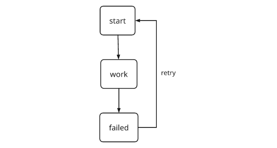
A waypoint that moves with the layout. In a inklet.graph edge mapping, a
bare (x, y) waypoint is millimetres in the frame the router sees -- the
laid-out graph's own, whose origin is its centre -- which is a number you have
to work out again every time a node is added. ("failed", "e") is the east
side of the node keyed failed, wherever the layout put it, and
(("failed", "e"), 6, 0) is 6mm clear of that side. Any key the graph accepts
works, and so does the node object itself.
STEPS = {"start": "start", "work": "work", "failed": "failed"}
EDGES = [("start", "work"), ("work", "failed"),
         ("failed", "start", {"waypoints": [(("failed", "e"), 6, 0)],
                              "label": "retry"})]
flow = inklet.graph({k: inklet.box(v) for k, v in STEPS.items()}, EDGES,
                 direction="down")
page = inklet.figure(width=90)
flow.add_to(page)
assert page.lint(rules=["LINK_CROSSES"]) == []
Rendered from the code above.
A label that reads over a busy panel
Three fields, one problem: a caption sitting on a mesh, a heatmap or a
photograph, where the ink is the same value as what is behind it. Fading the
whole node with opacity fades the caption too, and a white box behind the
words hides the data they are annotating.
fill_opacity and stroke_opacity fade a paint rather than a node, so a
tinted band can keep a solid edge; a halo is a stroke of the paper colour
painted under the letters, so the data shows through everywhere except the
half millimetre around each stem.
band = inklet.box(width=76, height=26, fill=TH.color(0), stroke=TH.color(0),
               fill_opacity=0.18, stroke_opacity=0.9, stroke_width=TH.stroke)
caption = inklet.text("peak 0.42 s", size=TH.font_size_small, halo=0.45)
panel = inklet.overlay([band, caption])

document = inklet.to_svg(panel)
assert 'fill-opacity="0.18"' in document       # the tint
assert 'stroke-opacity="0.9"' in document      # the edge, still legible
assert " opacity=" not in document             # and not the node as a whole
assert 'paint-order="stroke"' in document      # one pass, halo under the ink
The halo takes the page colour unless you name one, which is what you want on
the page and not what you want on a dark inset -- there, halo_color is the
colour the type is sitting on. A halo widens the space the label claims by
half its width on every side, so packing and the linter both already know
about it; you do not have to leave room by hand.
font_style="italic" both picks the italic face for the measurement and says
so in the file, so the label is italic in every spelling of the figure rather
than only in the one a browser re-shapes.
onto = inklet.text("−2.0 mm", size=TH.font_size_small, halo=0.45,
                halo_color=TH.paper, font_style="italic")

marked = inklet.to_svg(onto)
assert f'stroke="{TH.paper}"' in marked
assert 'font-style="italic"' in marked
assert "talic" in onto.prim.font_path          # measured in the italic face
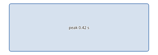
Rendered from the code above.
A PDF a reviewer can search
fig.to_pdf() outlines, which is right for a submission and means the file
has no text in it at all: no find box, no copy-paste, no screen reader.
text="embed" writes the same glyphs at the same places as real text, against
a subset of each face carried inside the file, plus the map that turns them
back into characters.
fig = inklet.figure(width="89mm")
fig.add(panel)

shipped = fig.to_pdf()
searchable = fig.to_pdf(text="embed")

assert b"/Subtype /Type0" in searchable and b"/ToUnicode" in searchable
assert b"/Subtype /Type0" not in shipped
assert searchable == fig.to_pdf(text="embed")  # byte-identical on a re-run
It is usually much smaller than outlining -- 45% to 86% off across the corpus figures, because a subset face costs once per alphabet where outlines cost once per letter -- and larger only on a figure with a handful of words on it. The trade is the other way round: an embedded PDF depends on the subset surviving whatever the destination does to the file, and some printer workflows may reject or alter embedded fonts. Outline for the journal, embed for the preprint server, the co-author and the lab wiki.
Two constraints apply. A face with CFF outlines cannot be a /FontFile2,
so blocks set in one are outlined and the rest of the page stays selectable;
this avoids refusing to write the file. A haloed
label is drawn as a stroked path under one text object rather than as two, so
searching the PDF finds each word once.
Three asterisks in a caption, and an italic n in the key
Two strings a figure legend always ends up wanting, both of which used to have to be worked around.
*** is how a caption names the p threshold the bracket over the bars is
drawing, and a caption in this house style already sets its panel letters
bold. A run of three or more asterisks is therefore never read as a
delimiter -- the grammar has no meaning for it, since bold is exactly ** and
italic is // -- so the convention and the panel letters coexist:
import inklet

caption = "**(a)** the assay. *** is p < 0.001 by permutation. **(b)** the fit."
marks = inklet.strip_markup(caption)

assert "*** is p < 0.001" in marks          # the stars survive
assert "**(a)**" not in marks               # the letters are still bold
For everything else there is \ -- it makes any one of * / { } | _ ^ \
literal -- and inklet.escape_markup to do it for a whole string, which is what
data interpolated into a caption should go through:
strain = "dpp**/+"
line = f"Genotype {inklet.escape_markup(strain)}, **n** = 12."

assert inklet.strip_markup(line) == "Genotype dpp**/+, n = 12."
A series name is prose too -- it is the caption for one curve -- so it reads
the same markup, which is the only way to get the italic n a style guide
insists on:
p = inklet.panel(width=60, height=38, x=(0, 8), y=(0, 100))
p.line([(x, 12 * x) for x in range(9)], name="ChR2 (//n// = 12)")
p.line([(x, 7 * x) for x in range(9)], name="eYFP (//n// = 11)")
p.axis("bottom", label="session")
p.axis("left", label="percent correct")
p.legend(corner="nw")

fig = inklet.figure(width=80, height=55)
fig.add(p.build())

assert 'font-style="italic"' in fig.to_svg()   # the n really is slanted
Pass legend(markup=False) for the other case: a name that came out of a
column header that contains literal // path separators.
A fold angle that differs between the parts of one scene
crease sets the minimum fold angle for drawing an edge. A smooth scanned
shell often needs a high threshold to omit tessellation edges; a small faceted
part may need a lower threshold to show its corners. Earlier scene rendering
used one threshold after fusing all parts, which could draw unwanted edges on
smooth surfaces.
Set crease in each part's options to preserve separate thresholds through
mesh fusion:
import inklet.three

shell = inklet.three.build("sphere", radius=1.0, subdivisions=2)
bead = inklet.three.build("box", size_x=0.4, size_y=0.4, size_z=0.4)
bead = bead.transformed(inklet.three.placement(at=(0.0, 0.0, 2.0)))

rig = inklet.scene([("shell", shell, {"crease": 120.0}),
                 ("bead", bead, {"crease": 20.0})],
                width=60, view="three-quarter", style="shaded",
                order="exact")

assert inklet.lint(rig) == []
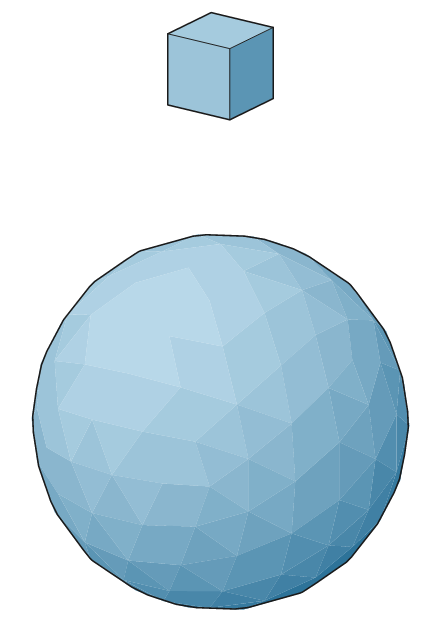
Rendered from the code above.
The shell's facet edges are omitted at 120 degrees and the bead's corners are
drawn at 20. Parts without their own angle use the scene's shared crease, as
they do for stroke_width.
An edge between two parts is tested against both thresholds. It is drawn if either part's threshold requires it, preserving edges where a low-threshold part meets a high-threshold part.
order="exact" resolves depth for overlapping facet pairs. It is the default
up to inklet.three.AUTO_EXACT_FACETS faces. Mean-depth sorting is faster but
can misorder intersecting or overlapping geometry.
Both files a paper needs, from one build
The PDF goes to the journal and the SVG stays open in the editor, and they
have to be the same picture: two calls means two builds, and a figure that
was laid out twice is a figure that can differ twice. save takes as many
paths as you have formats and writes them all from one build.
text says what the type in each file is, and the two formats do not offer
the same three. SVG takes "names" (the default -- a font-family chain),
"outline" or "embed"; PDF has no font-name mode and takes "outline"
(its default) or "embed". So text="embed" is the spelling that crosses
both, and it is what gets you a searchable PDF and a searchable SVG.
import inklet

fig = inklet.figure(width="89mm")
fig.add(inklet.text("Reaction yield against temperature"))

fig.save("figure.svg", "figure.pdf", text="embed")

assert b"FontFile" in open("figure.pdf", "rb").read()
assert "@font-face" in open("figure.svg").read()
"names" is an SVG answer to a question PDF does not ask, so a PDF written
under it outlines -- the safe reading of "I did not think about the PDF" --
while the SVG still gets its live <text>:
fig.save("chain.svg", "chain.pdf", text="names")

assert b"FontFile" not in open("chain.pdf", "rb").read()
assert "<text" in open("chain.svg").read()
Anything that is neither raises before a single file is written, rather than at whichever target happens to come first in the list:
import pytest

with pytest.raises(ValueError, match="unknown text mode"):
    fig.save("never.svg", "never.pdf", text="Embed")

import os
assert not os.path.exists("never.svg")
A row whose panels are not the same height
inklet.row lines panels up on their plot areas, not their boxes, which is
what keeps one panel's wide y numbers from shoving its data out of line with
its neighbour's. By default it puts the area centres on one line, which is
right when the areas are the same height and wrong the moment one member is
taller: a nested column of two panels centred among short neighbours rides
up half the difference, along with its panel letter.
align= picks the edge instead -- "top", "center" (the default,
"centre" too) or "bottom" for a row; "left", "center" or "right" for
a column.
import inklet

def panel(height):
    return (inklet.panel(30, height, x=(0, 1), y=(0, 1))
            .line([(0, 0), (1, 1)]).axes(x="t / s", y="dF/F"))

short, tall = panel(20), panel(34)

centred = inklet.row([panel(20), panel(34)], gap=5)
topped = inklet.row([panel(20), panel(34)], gap=5, align="top")

def area_tops(node):
    return [inklet.plot_area(member).y0 for member in node.children]

lo, hi = area_tops(centred)
assert abs(abs(hi - lo) - 7.0) < 1e-9      # half the 14mm difference
assert abs(max(area_tops(topped)) - min(area_tops(topped))) < 1e-9
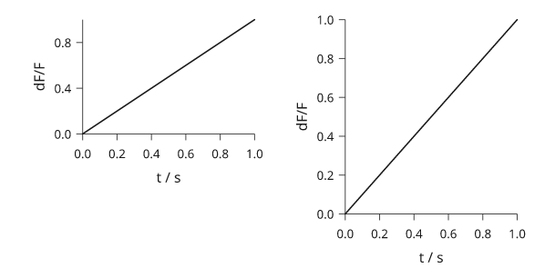
Rendered from the code above.
inklet.plot_area(node) is the reader, and it is public for exactly this: a
figure that composes panels by hand can ask where a node's data region is
instead of measuring its box. It answers in the frame node.bbox is in,
not the frame the rectangle was written in, and it follows the node:
built = short.build()
here = inklet.plot_area(built)
there = inklet.plot_area(built.translated(4, 9))

assert (there.x0 - here.x0, there.y0 - here.y0) == (4.0, 9.0)
assert inklet.plot_area(inklet.text("not a panel")) is None
The row itself declares the union of its members' areas, so a row inside a
column inside a row still lines up on data rather than on furniture:
inner = inklet.column([panel(20), panel(20)], gap=4)
outer = inklet.row([panel(34), inner], gap=5, align="top")

assert inklet.plot_area(outer) is not None
A layered graph that has to fit the column
A layered drawing comes out as wide as the layout makes it, and that is
usually narrower than the page. When it is not -- wider boxes, one more
branch -- the spill is boxes cut off at the page edge, which inklet.lint
reports as OFF_CANVAS. fit= tells the layout the width it has to come out
in, and it slides whole ranks sideways until the boxes are inside it:
import inklet

STEPS = {"load": "load reads", "trim": "adapter trim", "align": "align",
         "count": "count features", "norm": "normalise", "test": "DE test",
         "plot": "volcano plot", "table": "results table"}
EDGES = [("load", "trim"), ("trim", "align"), ("align", "count"),
         ("count", "norm"), ("norm", "test"), ("test", "plot"),
         ("test", "table"), ("load", "count")]

boxes = {key: inklet.box(text, width=26) for key, text in STEPS.items()}
loose = inklet.graph(boxes, EDGES, direction="down")
snug = inklet.graph(boxes, EDGES, direction="down", fit=inklet.COLUMN_SINGLE)

assert snug.width <= loose.width
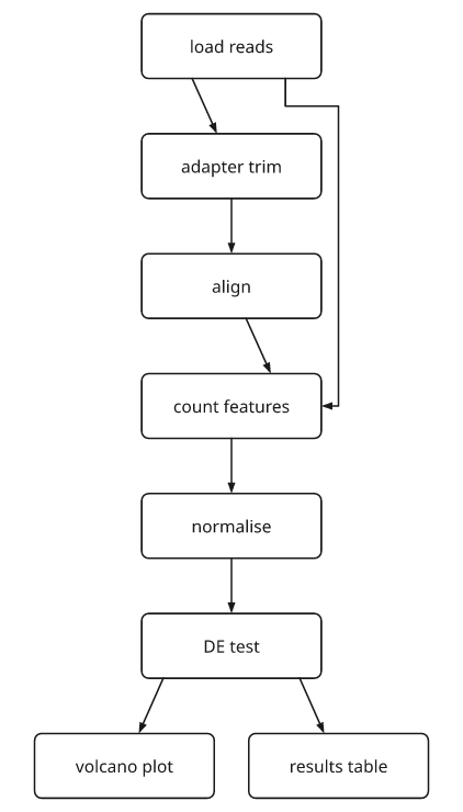
Rendered from the code above.
A fit wider than the existing graph leaves its width unchanged:
assert inklet.graph(boxes, EDGES, direction="down", fit=1000).width == loose.width
And it is not a guarantee. The ranks slide; they do not shrink, so a single rank wider than the limit stays wider than the limit and the drawing comes back too wide rather than with its boxes overlapping:
crammed = inklet.graph(boxes, EDGES, direction="down", fit=10)
assert crammed.width > 10
A page grid: laying finished panels out on a page
Use inklet.facets(..., axes=False) to align finished panels by their plot
areas. The axes=False option retains each panel's existing axes and other
plot furniture. Axis sharing and plot-area alignment are separate options.
inklet.grid instead aligns cells by their bounding boxes. A panel with a legend over it is taller at the top than
its neighbour, so aligning the boxes pushes its data area down by the height of
the legend, and a reader comparing the two panels is comparing two plots whose
frames do not agree:
def measured(name, key):
    q = inklet.panel(38, 24, x=(0, 10), y=(0, 10))
    q.line([(0, 1), (5, 6), (10, 9)], name=name)
    if key:
        q.line([(0, 2), (10, 8)], name="fit", stroke_dash=(1, 0.8))
        q.legend(side="top", columns=1)
    q.axes(x="t / s", y="signal")
    return q.build()

cells = [measured("wild type", False), measured("mutant", True),
         measured("rescue", False), measured("control", True)]

def area_tops(node):
    places = inklet.resolve(node)
    return [places[c.id].point("area-nw").y for c in cells]

aligned = area_tops(inklet.facets(cells, cols=2, axes=False, gap=6))
boxed = area_tops(inklet.grid(cells, cols=2, col_gap=6, row_gap=6))

assert aligned[0] == aligned[1]                 # one line, whatever is on top
assert abs(boxed[0] - boxed[1]) > 0.4           # the legend's height, as skew
Everything else on the page works the way it does inside a figure. inklet.letters
goes round the cells before the grid does, and letters a lettered panel off the
same plot area, so the letters share a baseline too:
page = inklet.facets(inklet.letters(cells), cols=2, axes=False, gap=6)
pagefig = inklet.figure(width="180mm")
pagefig.add(page)

assert pagefig.lint() == []
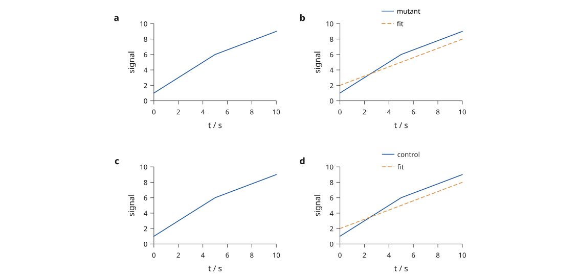
Rendered from the code above.
axes=False is not a lesser facets. cols, count, gap and the alignment
all behave the same; what goes is the shared x_label, y_label and the
thinning of the repeated tick numbers, which is right here because these panels
are not readings of one scale and each has to keep its own.
Drawing a protein
inklet.cartoon(chain) returns the ribbon a structural paper shows: a wide flat
band through each helix, an arrowed band along each strand, a thin round tube
everywhere else. It is a Mesh, so inklet.three.model draws it like any other
solid, and the faces come grouped by secondary structure -- "helix",
"strand", "coil" -- which is what colors= is keyed on.
It reads no file format. A residue, here, is anything with an alpha carbon
(ca), a DSSP letter (structure) and a number; a chain is anything with a
segments() that splits itself where the crystal lost the backbone. Whatever
your coordinates come out of -- a PDB reader, an mmCIF library, a trajectory
frame, a predicted model -- give it those three attributes rather than
converting into a type of ours:
import math
from inklet.three import Vec3, protein


class Residue:
    """Three attributes. That is the whole of what the cartoon reads."""

    def __init__(self, number, structure, ca):
        self.number, self.structure, self.ca = number, structure, ca


class Chain:
    """One list of residues per continuous run, in sequence order."""

    def __init__(self, runs):
        self.runs = runs

    def segments(self):
        return [list(run) for run in self.runs]


def a_helix(first, count):
    """2.3 A radius, 1.5 A rise, 100 degrees a residue -- an ideal alpha."""
    return [Residue(first + i, protein.HELIX,
                    Vec3(2.3 * math.cos(math.radians(100.0 * i)),
                         2.3 * math.sin(math.radians(100.0 * i)),
                         1.5 * i))
            for i in range(count)]


def a_strand(first, count, x):
    return [Residue(first + i, protein.STRAND,
                    Vec3(x, 0.6 * (-1) ** i, 3.3 * i))
            for i in range(count)]


chain = Chain((tuple(a_helix(1, 14)),
               tuple(a_strand(30, 8, 9.0))))       # a break between the two
fold = inklet.cartoon(chain)

assert fold.group_names == ("helix", "strand")
The two ends of this chain break are twenty angstroms apart. Connecting them
would add a segment absent from the supplied chain. cartoon sweeps each
segment separately and leaves the break unconnected.
This requires two non-default arguments, both derived from SIDES, the number
of points around the cross-section:
crease=45is above360 / SIDES. Below that the coil's own longitudinal seams are steeper than the threshold and get inked, and the protein comes out hatched.shading="smooth"because a tube sampled at a dozen points is a dozen flat strips, and flat shading paints all twelve however many tonelevelsit is given.
panel = inklet.three.model(fold, width=60, view="three-quarter",
                        style="shaded", shading="smooth", crease=45.0,
                        colors={"helix": "#c0504d", "strand": "#4f81bd",
                                "coil": "#b0b0b0"})

fig = inklet.figure(width="90mm")
fig.add(panel)

assert fig.lint() == []
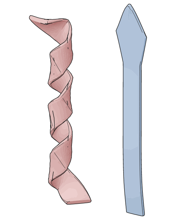
Rendered from the code above.
How finely to sample it is a question about the page, not about the
protein, so both answers are computed from the scale the model will be drawn
at. sides_for chooses the points round the section and steps_for the
cross-sections along the chain, both to a tolerance in millimetres on the
page -- and page_scale is how you get millimetres per angstrom before
committing to a mesh:
probe = inklet.cartoon(chain)                       # cheap, at the defaults
scale = inklet.three.page_scale(probe, width=60, view="three-quarter")

sides = protein.sides_for(scale, 0.06)
runs = [protein.ribbon(run, group=f"run-{run[0].number}", sides=sides,
                       steps=protein.steps_for(run, scale, 0.04))
        for run in chain.segments()]

assert sides >= protein.SIDES
assert all(1 <= n <= protein.STEPS
           for n in protein.steps_for(chain.segments()[0], scale, 0.04))
Ask steps_for for less than you ask sides_for. A section's departure from
its polygon is hidden inside a shaded surface; a spline's departure from its
chords lands on the silhouette, where a corner is about the most legible thing
a drawing has.
Every animal, and the statistics over them
For a small group, summary displays can conceal the number and arrangement of
observations. Boxplots show quartiles and violins estimate a smooth density;
consider overlaying or showing individual points so readers can assess the
sample directly. swarm draws one dot per observation and nudges them sideways
until none hides another:
CHR2 = [73.0, 74.1, 75.0, 77.9, 78.6, 80.0, 80.5, 83.0, 85.4, 92.5, 93.4, 99.0]
EYFP = [62.6, 62.8, 64.8, 66.1, 66.4, 67.6, 69.8, 70.4, 72.1, 74.6, 77.3]

scores = {"ChR2": CHR2, "eYFP": EYFP}
animals = inklet.panel(40, 34, x=list(scores), y=(55, 105))
animals.grid(x=False, y=True)
animals.swarm(scores, size=0.9, hollow=True)
for group, values in scores.items():
    mean = sum(values) / len(values)
    spread = sum((v - mean) ** 2 for v in values) / (len(values) - 1)
    animals.errorbars([(group, mean)], yerr=(spread / len(values)) ** 0.5)
animals.axes(y="session 8 correct (%)")

sheet = inklet.figure(width="60mm")
sheet.add(animals.build())
assert sheet.lint() == []
The layout adjusts only horizontal offsets: a dot is never moved along its value axis, so the mean and interval can be drawn over the very numbers the dots stand for. Nor is there a jitter to seed -- the placement is greedy and nearest-first over the values in order, so the same sample swarms the same way in every run and the SVG stays byte-identical.
When the swarm gets crowded, max_width= caps it in millimetres. The layout
reduces gaps before reducing marker size, using one size for the whole call even
when group sizes differ. For larger groups, put the swarm over the summary to
show both distribution and summary statistics:
both = inklet.panel(40, 34, x=list(scores), y=(55, 105))
both.boxplot(scores, width=0.5, outliers=False)
both.swarm(scores, size=0.8, max_width=7.0, color=[inklet.theme().muted] * 2)
both.axes(y="session 8 correct (%)")

page = inklet.figure(width="60mm")
page.add(both.build())
assert page.lint() == []
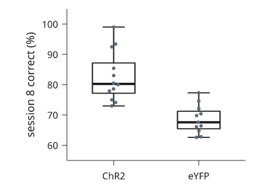
Rendered from the code above.
Cutting the empty middle out of an axis
Three colony counts are in the tens and one is in the hundreds. A linear axis
makes the smaller values difficult to compare; a log axis emphasizes ratios
rather than additive differences. A broken axis is another option when the
omitted range is disclosed. inklet.broken requires you to specify that range:
import inklet

STRAINS = ["wt", "cheA", "cheY", "fliC"]
COLONIES = [12, 31, 44, 385]

plate = inklet.panel(36, 32, x=STRAINS, y=inklet.broken((0, 400), breaks=[(45, 330)]))
plate.grid(x=False)
plate.bars(STRAINS, COLONIES)
plate.break_marks()
plate.axes(y="colonies")
breaks= specifies the omitted range. Both retained bands use the same
millimetres per unit. Ticks and gridlines are excluded from the omitted range,
even when explicitly requested, and the spine is interrupted. Automatic tick
spacing is refined so each retained band has a label.
break_marks() adds slashes to filled marks that cross the break. It leaves
other geometry, including thin whiskers, unchanged. Slashes identify the
omission but do not restore the original ratios between displayed bar lengths.
The linter reports the intentional difference between the displayed geometry and the numeric values:
paper = inklet.figure(width="60mm")
paper.add(plate.build())
codes = {d.code for d in paper.lint()}
assert codes == {"BREAK_DISTORTS"}
assert all(d.severity == "info" for d in paper.lint())
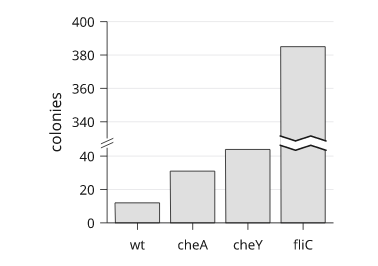
Rendered from the code above.
BREAK_DISTORTS has info severity. It reports filled marks crossing the gap
and marks on a shared baseline whose displayed lengths have altered ratios.
In this example, the bars for 385 and 31 have a displayed length ratio of about
3.4×, while their data ratio is 12.4×. Break marks do not remove the finding.
Disclose the omitted interval and consider a separate panel for the smaller values or a log axis. The log-axis example below produces no diagnostic findings:
logged = inklet.panel(36, 32, x=STRAINS, y=inklet.log((10, 1000)))
logged.grid(x=False)
logged.bars(STRAINS, COLONIES, baseline=10)
logged.axes(y="colonies")

sheet = inklet.figure(width="60mm")
sheet.add(logged.build())
assert [d.code for d in sheet.lint()] == []
A log axis cannot include zero. This example explicitly uses a baseline of 10, so bar lengths represent logarithmic distances from 10, rather than counts from zero. State the baseline and choose the scale for the comparison readers need to make.
Forty labels and nowhere to put them
inklet.annotate places each label using the obstacles present when it is
called. Later labels may compete for the same space, producing overlaps or
crossing leaders in dense figures. A subsequent placement pass can consider
the completed drawing.
First construct and label the figure normally:
import inklet

TH = inklet.use_theme("nature")
FIELD = [(2.0, 2.0, "alpha"), (9.0, 3.0, "beta"), (16.0, 2.5, "gamma"),
         (4.0, 9.0, "delta"), (10.5, 8.0, "epsilon"), (15.0, 9.5, "zeta"),
         (3.0, 15.0, "eta"), (11.0, 15.5, "theta"), (17.0, 14.0, "iota")]

cells = inklet.place([((x, y), inklet.marker("circle", 1.2, fill=TH.ink,
                                       stroke="none").named(name))
                   for x, y, name in FIELD])
crowded = cells
for _, _, name in FIELD:
    crowded = inklet.annotate(cells.find(name), name, within=crowded, clear=1.0,
                           size=TH.font_size_small)
fig.lint() reports these findings:
before = inklet.figure(width="72mm", theme=TH, margin=4)
before.add(crowded)
noisy = [d.code for d in before.lint()
         if d.code in ("CROWDING", "OVERLAP", "LINK_CROSSES")]
assert noisy, "the fixture is meant to be crowded"
inklet.place_labels is the other end of that loop. It peels the annotations off,
scores all eight compass sides at two clearances for every label against the
marks, the labels already placed and the leaders already drawn, and rebuilds
the tree with the winners:
tidy = inklet.place_labels(crowded)

after = inklet.figure(width="72mm", theme=TH, margin=4)
after.add(tidy)
assert [d.code for d in after.lint()
        if d.code in ("CROWDING", "OVERLAP", "LINK_CROSSES")] == []
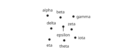
Rendered from the code above.
Two properties make it safe to leave in a script. It is a fixed point — running it again changes nothing, so a build that calls it twice is not a bug:
assert inklet.place_labels(tidy) == tidy
— and it does not depend on the order you wrote the labels in, only on
where their targets sit in the frame, so a loop over a dict and a loop over a
sorted list produce the same figure. Read the decision back with
inklet.label_plan, which answers without building anything:
plan = inklet.label_plan(crowded)
assert sum(choice.moved for choice in plan) >= 3
assert not any(choice.moved for choice in inklet.label_plan(tidy))
It is opt-in and narrow on purpose: v1 moves point-labels with leaders, and
leaves panels, ticks, axis labels and legends to the things that own them. A
tree with no annotate in it comes back as the very same object.
A flow whose width is the measurement
A Sankey is the one drawing where the thickness of a line is the datum, so
the layout has more to get right than a graph does: one scale for the whole
page, a bar as tall as what goes through it, and ribbons that tile a node face
with no gap and no overdraw. inklet.sankey takes (source, target, value)
triples and decides all of it -- the column order included.
import inklet

FATE = [
    ("cohort", "ipc", 420), ("cohort", "org", 250), ("cohort", "glia", 210),
    ("glia", "astro", 130), ("glia", "oligo", 70),
    ("ipc", "deep", 150), ("ipc", "upper", 240),
    ("org", "upper", 170), ("org", "deep", 60),
]
fates = inklet.sankey(FATE, length=110, breadth=48,
                   labels={"ipc": "intermediate\nprogenitor",
                           "org": "outer radial\nglia"})

sheet = inklet.figure(width="120mm", theme="nature", margin=4)
sheet.add(fates.diagram)
assert sheet.lint() == []
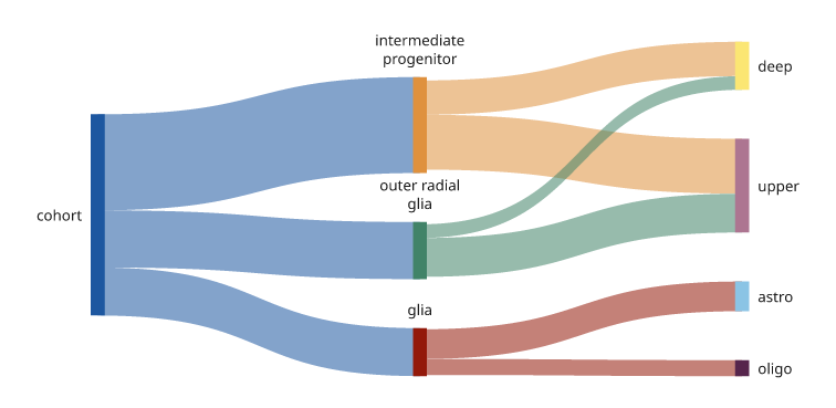
Rendered from the code above.
The rank of a node comes from the flows, and so does its height: every bar is
max(inflow, outflow) tall at one shared scale, chosen so the busiest column
fills the breadth you gave. length is the whole drawing including the end
labels, so a Sankey asked for a column's width fits that column rather than
hanging its names off the page.
The order within a column is a crossing-minimisation problem, and this one is
a stated greedy: barycentre sweeps, then adjacent swaps while a swap helps,
scored by counting the ribbons that actually cross. order="given" turns it
off, which is how the improvement gets measured rather than asserted:
assert inklet.sankey(FATE, length=110, breadth=48, order="given").crossings == 9
assert fates.crossings == 1
Two numbers come back for the caption. crossings is that count, and unit is
the millimetres one unit of value came out as -- which is what a scale key has
to be drawn from if it is not to drift out of step with the figure:
key = inklet.bracket((0, 0), (0, 100 * fates.unit), text="100 cells", side="e")
assert key.height == 100 * fates.unit
Handles survive the layout, so a bar can be annotated after the fact.
annotate returns the target's whole tree with the callout added, so the
annotated drawing is what goes on the figure -- adding fates.diagram as well
would place it twice:
called = inklet.annotate(fates["upper"], "most of the cohort", side="e",
                      clear=2.0, within=fates.diagram)
sheet = inklet.figure(width="120mm", theme="nature", margin=4)
sheet.add(called)
assert fates["upper"].id in inklet.resolve(called)
tint="target" colours each band by where it ends
rather than where it starts, which is the right choice when the first column is
one undifferentiated pool and colouring by source would paint every band the
same grey. direction="down" turns the whole picture a quarter turn.
A dial, a rose, and the arrow that says how tuned the cell is
inklet.polar is inklet.panel with the rectangle replaced by a disc. The number
you pass is the radius of the data region, so the finished node is wider than
that: the theta labels, the r labels and any key stand outside the rim, exactly
as a rectangular panel's axes stand outside its box.
Two arguments settle the convention, and settling them here is the point of the
call -- a polar figure built on the wrong one is wrong without looking wrong.
zero= is where theta 0 points on the page ("up", "east", or a number of
page degrees), and winding= is which way the data runs from there: "ccw" is
the mathematical default and "cw" is what a compass, a clock and a
head-direction rig all use.
import inklet

TUNING = [(a, 2 + 9 * (1 + __import__("math").cos(
    __import__("math").radians(2 * (a - 40))))) for a in range(0, 360, 15)]

cell = inklet.polar(20, r=(0, 24), zero="up", winding="cw")
cell.grid(r_count=3, theta_count=8)
cell.line(TUNING, name="cell 41")
cell.scatter(TUNING, size=0.9, name="cell 41")
cell.mean_vector([a for a, _ in TUNING], [v for _, v in TUNING], order=2)
cell.theta_axis(count=8, label="drift direction")
cell.r_axis(at=292.5, count=3, label="spikes s⁻¹")

sheet = inklet.figure(width="80mm", theme="nature", margin=3)
sheet.add(cell.build())
assert sheet.lint() == []
The segments between samples are arcs, not chords: a tuning curve sampled
every 30 degrees and joined with straight lines is a dodecagon, and a reader
cannot tell its flat sides from a plateau in the data. interpolate=False gets
the chords back for a polygon of measured vertices.
mean_vector draws the circular mean as an arrow from the pole whose length
is the resultant R, with R = 1 reaching the rim. order=2 is the orientation
statistic, and a figure about gratings, dendrites or fibre alignment needs it:
a cell answering equally at 40 and 220 degrees is perfectly oriented and has no
direction at all, so order=1 reports R = 0 -- correctly, and uselessly. The
same two numbers come back for the caption:
axis_angle, selectivity = inklet.circular_mean(
    [a for a, _ in TUNING], [v for _, v in TUNING], order=2)
assert round(axis_angle) == 40
assert 0.4 < selectivity < 0.6
An arrow too short to fit its arrowhead is drawn as a dot at the pole instead. That is deliberate: a triangle with no shaft reads as a large resultant pointing nowhere, which is the opposite of what the sample says.
A rose is the same panel with rose() instead of a line, and
circular_histogram bins the angles for it -- wrapping round the turn, which
is the difference between it and inklet.histogram and the reason a wind rose
cannot be built from the rectangular one. Orientation data lives on the half
turn, so the panel is a fan:
import random

rng = random.Random(7)
preferred = [rng.gauss(rng.choice((0.0, 90.0)), 17.0) % 180.0 for _ in range(220)]
centres, counts = inklet.circular_histogram(preferred, bins=18, domain=(0, 180))

rose = inklet.polar(20, r=(0, max(counts)), theta=(0, 180), hole=2.0)
rose.grid(r_count=2, theta_count=6)
rose.rose(counts, at=centres, width=0.94, name="cells")
rose.theta_axis(count=6, label="preferred orientation")
rose.r_axis(count=2, label="cells", plate=False)

sheet = inklet.figure(width="80mm", theme="nature", margin=3)
sheet.add(rose.build())
assert sheet.lint() == []
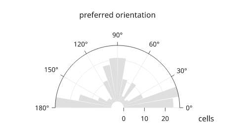
Rendered from the code above.
Ticks come off an angular lattice, not the 1/2/5 one: whole divisors of a
turn, so an axis is labelled every 30 degrees or every π/4 and never every 0.7
radians. Radian panels are written as fractions of π for the same reason --
1.5707963 on an axis is a number the reader has to decode:
dial = inklet.polar(14, r=(0, 1), theta=(0, 2 * 3.141592653589793), unit="rad")
dial.grid(r_count=2, theta_count=8).theta_axis(count=8).r_axis(count=2)
labels = dial.theta.labels(dial.theta.ticks(8))
assert "π/4" in labels and "3π/2" in labels
The ticks stay when the labels thin. A rectangular axis drops a tick with
its label, because along a straight axis an unlabelled tick is a value the
reader cannot name. On a circular axis, retaining tick marks while thinning
labels preserves angular positions; keeping twenty-four marks while labelling
twelve is useful for dense directional displays. theta_axis(curved=True) sets those
numbers along the rim instead of upright, which is useful on a dial with long
labels; which labels survive the thinning does not change either way.
A PolarPanel is not a Panel, so pass its build() to inklet.row and
inklet.column. It publishes the same two notes a rectangular panel does -- the
plot area and the r domain -- so inklet.letters, OFF_PANEL and KEY_MISMATCH
keep working without knowing the module exists:
both = inklet.row(inklet.letters([cell.build(), rose.build()]), gap=8, align="top")
assert inklet.plot_area(cell.build()).width == 40.0
Type that follows the line
Two ways to set a run somewhere other than horizontally, and one convention
that governs both: degrees are clockwise on the page, because y grows
downward. angle=90 reads top-to-bottom; use angle=-90 for a y-axis label
that reads bottom-to-top:
import inklet

sideways = inklet.text("fluorescence / a.u.", size=2.6, angle=-90)
assert sideways.bbox.height > sideways.bbox.width
The whole shaped block turns, not the letters one at a time, and the envelope
turns with it -- so a stack, a inklet.lint clearance and a Figure.report all
measure the rotated extent rather than the box the type would have had lying
down.
For a run that follows a curve, hand inklet.text_on_path the very node the
figure draws. It takes the node's own cubics, so the type lands on the curve
the backend strokes rather than a flattened approximation, and it retains the curve's
origin, which is what keeps inklet.drawn([...]) in register:
spiral = inklet.curve([(-24, 6), (-8, -8), (8, -8), (24, 6)],
                   stroke="#9aa0a6", stroke_width=0.3)
along = inklet.text_on_path("excitation sweep", spiral, size=2.6, lift=0.9)

page = inklet.figure(width="90mm", margin=4)
page.add(inklet.drawn([spiral, along], kind=inklet.abutting("annotation")))
assert page.lint() == []
Two things earn their keep in those three lines. lift= is one: with the
baseline sitting on a curve the figure also draws, the stroke runs through
the letters and PATH_CROSSES says so, correctly -- about a third of the type
size is enough to clear it. side="below" hangs the run under the curve
instead, the same way up.
inklet.abutting is the other. Type set along a line is meant to be nearer to
it than the millimetre of clearance CROWDING asks of two unrelated things,
so the pair is a description of the drawing rather than a finding, and the
library's answer to that is a declaration and never a tolerance: lowering
min_clearance_mm would silence the tick label two tenths of a millimetre off
its axis on the same page.
Round a circle, inklet.text_on_arc does the radius arithmetic. side is named
for the circle -- "outside" keeps the ink clear of radius on the far side
from the centre, by gap millimetres -- and the run turns itself over on the
half of the ring where it would otherwise read upside-down, so a whole set of
labels comes out legible without the caller working out which half each is on:
rim = inklet.arc(19, -180, 179.99, stroke="#9aa0a6", stroke_width=0.3)
ring = [inklet.text_on_arc(word, 19, bearing, size=2.4, gap=0.8)
        for word, bearing in (("anterior", -90), ("left", 180),
                              ("posterior", 90), ("right", 0))]
sheet = inklet.figure(width="70mm", margin=4)
sheet.add(inklet.drawn([rim, *ring], kind=inklet.abutting("compass")))
assert sheet.lint() == []
Rendered from the code above.
The result has three relevant properties. Each shaping cluster becomes its
own live text node, so save(text="embed") still writes words a reader can
select and search -- one <text> per cluster, in reading order -- and the
whole string is recorded on the group where a diagnostic can quote it. A run
longer than its curve continues straight along the exit tangent and visibly
overruns; pass overflow="raise" if you are generating labels in a loop and
would rather be told. And each letter turns about the middle of its own body
rather than about its baseline, which is what stops the insides of the letters
pinching on a tight curve -- pivot=0 restores the naive placement if you want
to see the difference.