On this page

Dense data¶

Choose how each data layer is represented. The rest of the figure can retain vector axes, labels, annotations and legends regardless of that choice.

Layer	Option	What changes
Dense point cloud	`scatter(..., raster=True, dpi=300)`	Markers become one raster layer; point order and opacity are retained
Regular matrix	`matrix(..., raster=True)`	Cells become an image; the colour scale still supplies a vector colorbar
Dense straight line	`line(..., simplify=0.02)`	Optional reduction of vector vertices within a physical tolerance
Every authored vector point	Omit `simplify`, or use `simplify=0`	Every line vertex is retained

Raster scatter requires Pillow (pip install 'inklet[images]'). Raster matrices use Inklet's standard-library PNG encoder, so creating the matrix and saving it as SVG do not require Pillow. Saving that embedded image to PDF does require Pillow (images or render). PNG export additionally needs the render extra. Vector line simplification is part of the core package. Install extras in the environment that runs the script, for example .venv/bin/pip install 'inklet[images,render]'.

Scatter layers with at least 256 points use packed vector markers automatically; they remain editable and retain every observation. Use raster=True when a single image layer is preferable. Matrix raster='auto' switches around 2,000 cells; see Matrices for vector='batched', vector='seamless', missing values and interpolation choices.

Rasterise a dense mark layer¶

Each vector marker is written as its own shape, about 150 bytes of SVG. A layer of tens of thousands of markers therefore makes a file of several megabytes that an editor opens slowly, while the same layer as one image is tens of kilobytes. In one measured figure, 72,000 small filled squares in a 170 mm panel gave a 10.9 MB SVG as vectors and 30 KB with raster=True.

Rasterise a layer when it has thousands of markers, especially small filled squares or glyphs that overlap, and when no one needs to select or edit the markers one at a time in the vector file:

import inklet as i

points = [(k / 100, (k * 37 % 1000) / 1000) for k in range(36000)]
p = i.plot_spec(x=(0, 360), y=(0, 1), height=40)
p.scatter(points, marker='square', size=0.8, color='#000000', raster=True, dpi=300)
p.axes(x='Position', y='Density')
doc = i.document(width=170)
doc.add('density', p)
doc.save('density.svg')

Keep a layer vector when it has few markers, when each marker must stay editable, or when its outlines are dashed, since an image cannot draw a dash. Only the marker layer becomes an image; axes, labels, the key and other layers stay vector.

The full model's Panel.scatter keeps every layer vector unless raster=True. Quick charts switch to an image past 20,000 points per panel, as quick charts describes.
Lint does not warn about file size and does not suggest raster=True, so check the output yourself, for example with len(figure.to_svg()).

Reduce vector line geometry¶

import math
import inklet as i

points = [(k/1000, math.sin(k/1000)) for k in range(20001)]
p = i.plot_spec(x=(0, 20), y=(-1.1, 1.1), height=40)
p.line(points, simplify='0.02mm', stroke='#176b9b')
p.axes(x='Time / s', y='Response')
doc = i.document(width=120)
doc.add('signal', p)
doc.save('signal.svg', 'signal.pdf')

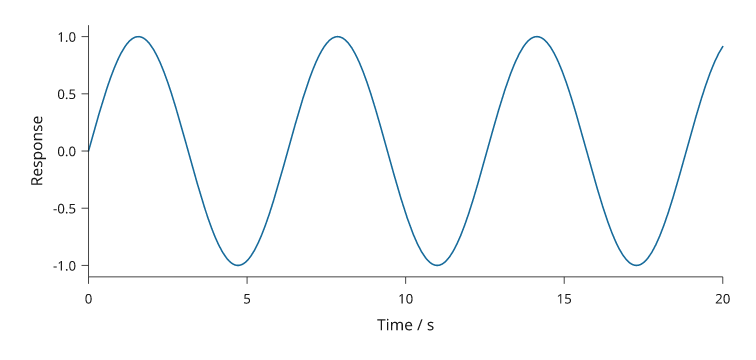
Twenty thousand sinusoid samples rendered with a 0.02 mm line tolerance

Rendered from the code above.

The tolerance is applied after mapping through the plot scales, including logarithmic scales. Every removed vertex is within that distance of the segment that replaces it. Endpoints and global x/y extrema are retained. A resized live plot recomputes the reduction at its new physical size.

This is an explicit rendering approximation. It can remove details smaller than the chosen tolerance and change the phase of dashed strokes. It does not change the dataset or perform statistical smoothing. Uncertainty bands and error bars retain their own complete geometry. Use it for straight, open lines; combining positive simplification with smooth or closed=True raises an error. Coordinates must be finite. Validate the reduced export at its final physical size, especially where a sharp peak, crossing, or narrow interval matters to the interpretation. Keep an unsimplified archive when the figure is used for measurement or digitization.

The reducer limits its work on difficult paths by retaining additional vertices. It does not increase the tolerance to satisfy a point-count target. Each reduced line records line_simplification in its diagram notes, including the input and output point counts and tolerance.

Inspect the result¶

Compare the plot rendering review and its zoomed specimen. The rendering engine measurements cover raster scatter, repeated images and document layout. Measure your own workload: constructing layers, compiling a document and writing exports have different costs.

Keep manuscript captions outside the artwork. Record any approximation or raster resolution needed to interpret or reproduce the figure in that caption.