On this page

Dense figure pages¶

A journal figure page often holds a dozen small panels at 183 mm wide: a schematic, bar charts with counts, heatmaps, cumulative distributions, a radar chart and a donut. The scientific.cell preset sets the type sizes, strokes and spacing for such a page, and a 12-column document places the panels.

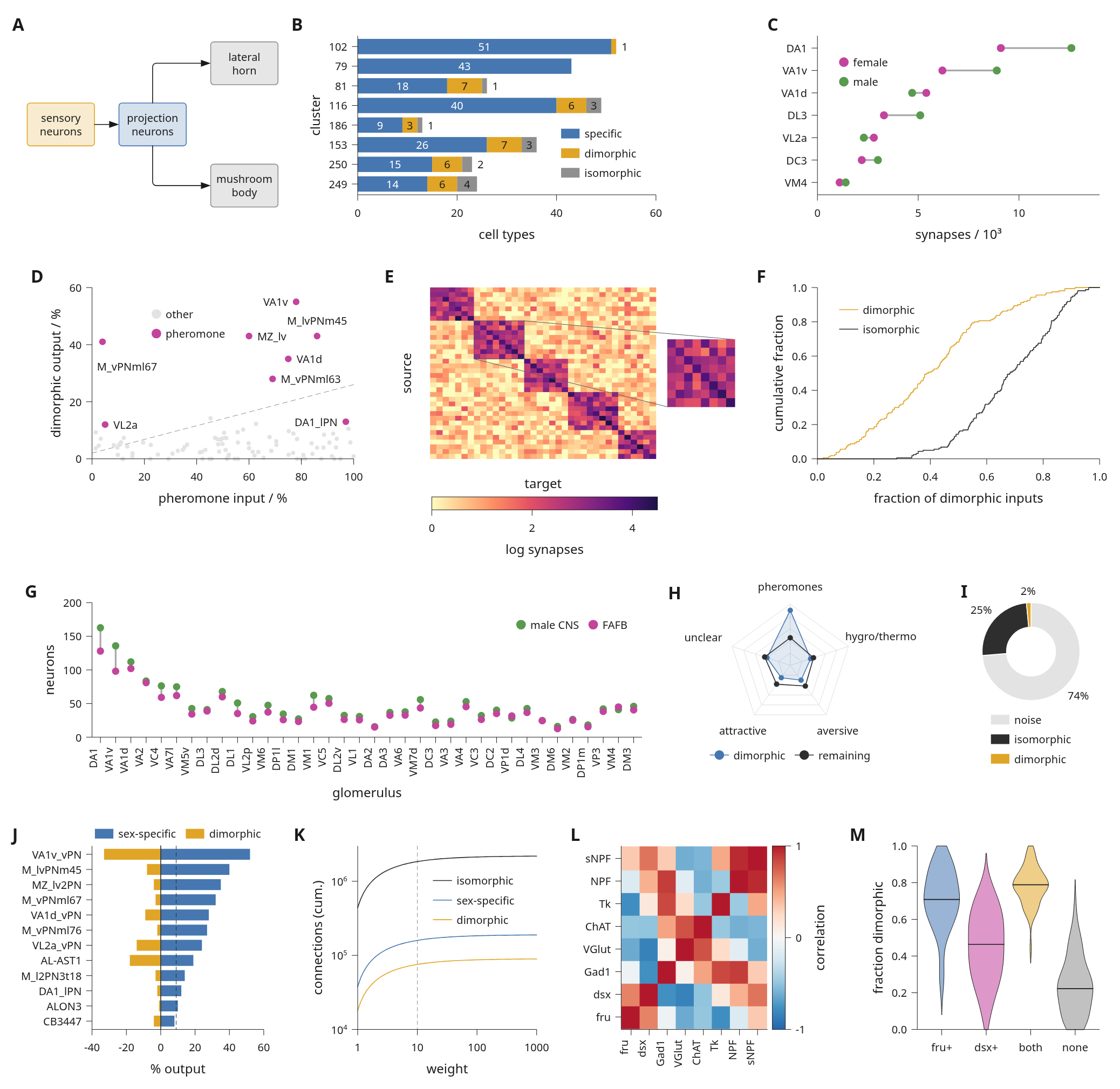
A thirteen-panel figure page: circuit diagram, stacked bars with counts, dumbbells, labelled scatter, heatmap with a zoom inset, cumulative distributions, a dot plot over 36 categories, radar, donut, diverging bars, a log-log plot, a correlation matrix and violins

The figure above is examples/dense_figure.py. All data are simulated. It compiles to SVG, PDF and PNG, and prints the lint report for the page.

What each panel uses¶

Panel	Content	Calls
a	Circuit schematic	`composition()`, `module()`, `link(route='orthogonal')`; see diagrams
b	Stacked horizontal bars with counts	`bars(stacked=True, orient='h', labels=True)`; see bar value labels
c	Two groups per category	`dumbbell()`; see dumbbells
d	Scatter with named points	`scatter()`, `label_points()`; see labelled points and label placement
e	Heatmap, colour bar and zoom inset	`matrix()`, `colorbar()`, `inset(zoom=...)`; see heatmaps
f	Cumulative distributions	`ecdf()`; see cumulative distributions
g	Dot plot over 36 categories	`dumbbell()` with rotated tick labels
h	Radar chart	`polar().radar_grid()`, `radar()`; see radar charts
i	Donut	`polar(hole=...)`, `pie()`; see pie and donut charts
j	Diverging bars	two `bars(orient='h')` layers and `vline(0)`
k	Cumulative counts on log axes	`line()` with `x=i.log(...)`, `y=i.log(...)`
l	Correlation matrix	`matrix(center=0)` with a diverging ramp
m	Violins	`violin()`; see violins

The page grid¶

The document has 12 columns and four rows. Each panel spans a number of columns; row heights come from the tallest plot in the row. The example sets share_plot_margins=True, so data edges line up along shared grid lines while each row keeps its own plot height. Panel letters are added by .letters() in the order the panels are added.

import inklet as i

style = i.preset('scientific.cell')
blue, amber, magenta, grey, green, ink = style.theme.palette

types = ['DA1', 'VA1v', 'VA1d', 'DL3']
pairs = i.plot_spec(height=26, x=(0, 14), y=types[::-1])
pairs.dumbbell(types, [[9.1, 6.2, 5.4, 3.3], [12.6, 8.9, 4.7, 5.1]], orient='h',
               name=['female', 'male'], color=[magenta, green])
pairs.axes(x='synapses / 10³')
pairs.legend()

samples = [k / 40 for k in range(41)]
cumulative = i.plot_spec(height=26, x=(0, 1), y=(0, 1))
cumulative.ecdf([s ** 2 for s in samples], name='dimorphic', stroke=amber)
cumulative.ecdf(samples, name='isomorphic', stroke=ink)
cumulative.axes(x='fraction of inputs', y='cumulative fraction')
cumulative.legend()

points = [(78, 55), (60, 43), (86, 43), (5, 12)]
named = i.plot_spec(height=26, x=(0, 100), y=(0, 60))
named.scatter(points, size=1.1, color=magenta)
named.label_points(points, ['VA1v', 'MZ_lv', 'M_lvPNm45', 'VL2a'])
named.axes(x='pheromone input / %', y='output / %')

doc = style.document(columns=12).letters()
doc.add('pairs', pairs, row=0, column=0, colspan=4)
doc.add('cumulative', cumulative, row=0, column=4, colspan=4)
doc.add('named', named, row=0, column=8, colspan=4)
figure = doc.compile()
figure.save('dense-row.svg', 'dense-row.pdf')
assert not [d for d in figure.lint() if d.severity == 'error'], figure.report()

Widths are physical: at 183 mm with a 2 mm margin and 3.5 mm gaps, a 4-column span is about 57 mm. Axis labels, tick labels and legends are measured with the embedded font before each data region is placed, so panels in the same row keep aligned data areas even when their tick labels differ in length.

What the preset changes¶

scientific.cell uses 6 pt body text, 5 pt tick labels, 8 pt bold panel letters, 0.4 pt axes and 0.25 pt hairlines. Legends without an explicit side go inside the data area, in space that no mark occupies. The lint thresholds follow the preset: a 5 pt minimum text size and a 0.25 pt minimum stroke. The full table is in presets: dense pages.

Run the complete example¶

From a repository checkout:

python examples/dense_figure.py

It writes out/dense-figure/figure.svg, .pdf and .png, and prints the diagnostics. See export and review for what the findings mean, and panel layout for spans, nested subfigures and fixed artwork.