Distributions and individual samples¶

A histogram groups observations into bins; boxplots summarize quartiles; violins estimate a smooth density; swarms retain the individual values. State the sample population and any grouping or smoothing used.

All values below are illustrative simulated observations. Each snippet can be run independently with core Inklet; PNG preview generation additionally uses the render extra. Run a block from the repository root with .venv/bin/python; each block writes an SVG and PDF. These methods summarize the values you pass and do not perform a statistical test.

Choose a display from the question: a histogram shows bin counts, a boxplot shows robust summaries, a violin shows a smoothed shape, and a swarm shows individual observations. Keep group sample sizes visible in the caption.

Histograms¶

Histograms count observations within explicit bins. density=True divides by sample size and bin width so the bar area integrates to one. Use inklet.plot.histogram first when the counts should determine the y domain. Bin edges affect the displayed distribution, so report them or the rule used to choose them. Unequal bin widths need particular care when comparing bar heights.

import inklet as i
import random
rng = random.Random(401)
values = [rng.gauss(3.0, .62) for _ in range(96)]
from inklet.plot import histogram
edges, counts = histogram(values, bins=[n / 2 for n in range(13)])
p = i.plot_spec(x=(0, 6), y=(0, max(counts) + 4), height=44)
p.hist(values, bins=edges, color='#24698c', stroke='white', stroke_width=.15)
p.grid(x=False, y=True, count=5, stroke='#e1e7e4', stroke_width=.15)
p.axes(x='Duration / s', y='Count')
doc = i.document(width=110)
doc.add('hist', p)
doc.save('hist.svg', 'hist.pdf')

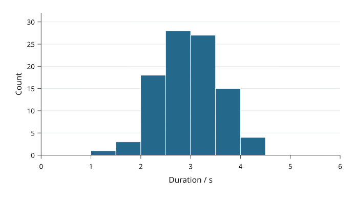
Rendered from the code above. Ninety-six simulated durations are grouped into 12 half-second bins; the bars show counts, not a fitted distribution.

Counts that are already binned. hist bins whatever it is given, so a table of counts per bin, such as a source-data file, would be counted again. prebinned=True draws the counts as they are: values are the counts, and bins the edges, one more than the counts. orient='h' turns the bars across the page, for a marginal beside a 2D plot, and density=True divides the counts by their total and by each bin's width.

import inklet as i
p = i.plot_spec(x=(0, 1), y=(0, 120), height=44)
p.hist([12, 40, 88, 61], bins=[0, .25, .5, .75, 1], prebinned=True, color='#24698c')
p.axes(x='Fraction', y='Count')
doc = i.document(width=110)
doc.add('binned', p)
doc.save('binned.svg', 'binned.pdf')

Boxplots¶

Boxplots show the median, quartiles and Tukey whiskers. Whiskers stop at the furthest observation within whisker times the interquartile range. More distant observations are shown separately by default. The box does not show sample size or the full distribution. Overlay a swarm for small groups, and do not interpret whisker points as automatically erroneous.

import inklet as i
import random
rng = random.Random(402)
samples = {'Control': [rng.gauss(4.1, .62) for _ in range(72)],
           'Treated': [rng.gauss(4.65, .78) for _ in range(72)]}
p = i.plot_spec(x=['Control', 'Treated'], y=(1, 8), height=44)
p.boxplot(samples, color=['#24698c', '#288675'])
p.grid(x=False, y=True, count=5, stroke='#e1e7e4', stroke_width=.15)
p.axes(y='Measurement / a.u.')
doc = i.document(width=110)
doc.add('boxplot', p)
doc.save('boxplot.svg', 'boxplot.pdf')

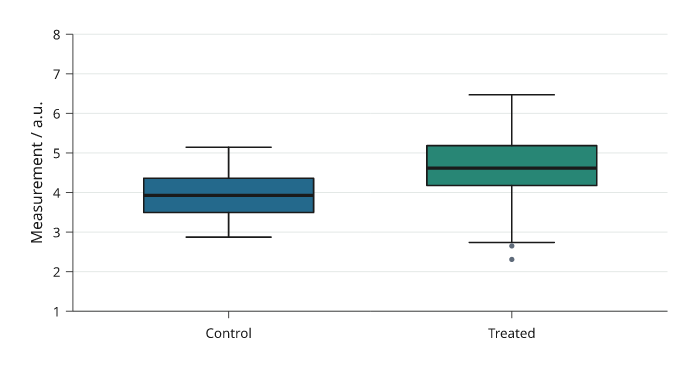
Rendered from the code above. The same 72 simulated observations per group are reduced to quartiles and Tukey whiskers; sample size is not encoded by box width.

Violins¶

Violins show a kernel-smoothed sample distribution. The default bandwidth follows Silverman’s robust rule; bandwidth, cut and samples control smoothing and drawing extent. For small groups, showing the individual observations can reveal more than a smooth outline. The density is an estimate, so bandwidth can create or remove apparent modes; report the selected bandwidth when the shape supports a substantive claim.

import inklet as i
import random
rng = random.Random(402)
samples = {'Control': [rng.gauss(4.1, .62) for _ in range(72)],
           'Treated': [rng.gauss(4.65, .78) for _ in range(72)]}
p = i.plot_spec(x=['Control', 'Treated'], y=(1, 8), height=44)
p.violin(samples, color=['#24698c', '#288675'], cut=1.5)
p.grid(x=False, y=True, count=5, stroke='#e1e7e4', stroke_width=.15)
p.axes(y='Measurement / a.u.')
doc = i.document(width=110)
doc.add('violin', p)
doc.save('violin.svg', 'violin.pdf')

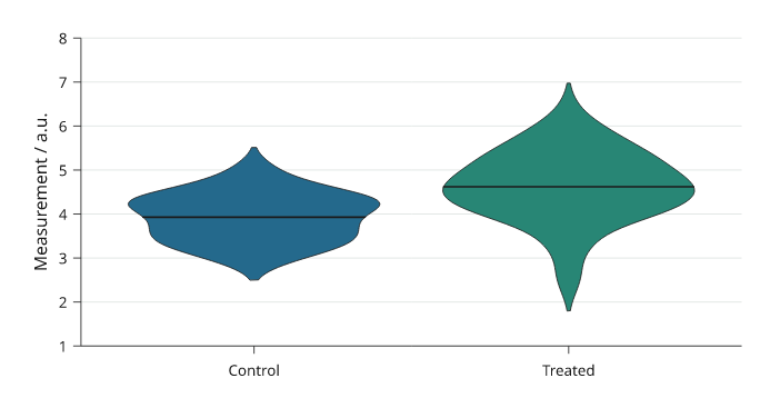
Rendered from the code above. These violins use the same 72 observations as the boxplots; their outlines are bandwidth-dependent density estimates.

Swarms¶

Swarms show every observation, including repeated values. Only the sideways placement changes to separate markers. The measured value stays fixed. size is marker diameter in millimetres; crowded groups may need more panel width or smaller markers.

import inklet as i
import random
rng = random.Random(402)
samples = {'Control': [rng.gauss(4.1, .62) for _ in range(72)],
           'Treated': [rng.gauss(4.65, .78) for _ in range(72)]}
p = i.plot_spec(x=['Control', 'Treated'], y=(1, 8), height=44)
p.swarm(samples, size=1.0, color=['#24698c', '#288675'])
p.grid(x=False, y=True, count=5, stroke='#e1e7e4', stroke_width=.15)
p.axes(y='Measurement / a.u.')
doc = i.document(width=110)
doc.add('swarm', p)
doc.save('swarm.svg', 'swarm.pdf')

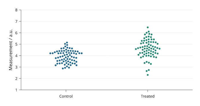
Rendered from the code above. Every point is one of the same 72 observations per group used above; only its horizontal position is adjusted to separate overlapping points.

Cumulative distributions¶

ecdf draws the empirical cumulative distribution: the fraction of observations at or below each value, as a step line. Every observation is shown and no bin width or bandwidth is chosen. complementary=True draws the fraction above each value instead. normalize=False draws counts. inklet.plot.ecdf(values) returns the steps without drawing them.

import inklet as i
import random

rng = random.Random(402)
control = [rng.gauss(4.1, .62) for _ in range(72)]
treated = [rng.gauss(4.65, .78) for _ in range(72)]
p = i.plot_spec(x=(1, 8), y=(0, 1), height=44)
p.grid(x=False, count=4, stroke='#e1e7e4', stroke_width=.15)
p.ecdf(control, name='Control', stroke='#24698c', stroke_width=.45)
p.ecdf(treated, name='Treated', stroke='#288675', stroke_width=.45)
p.axes(x='Measurement / a.u.', y='Cumulative fraction').legend(side='bottom')
doc = i.document(width=110)
doc.add('ecdf', p)
doc.save('ecdf.svg', 'ecdf.pdf')

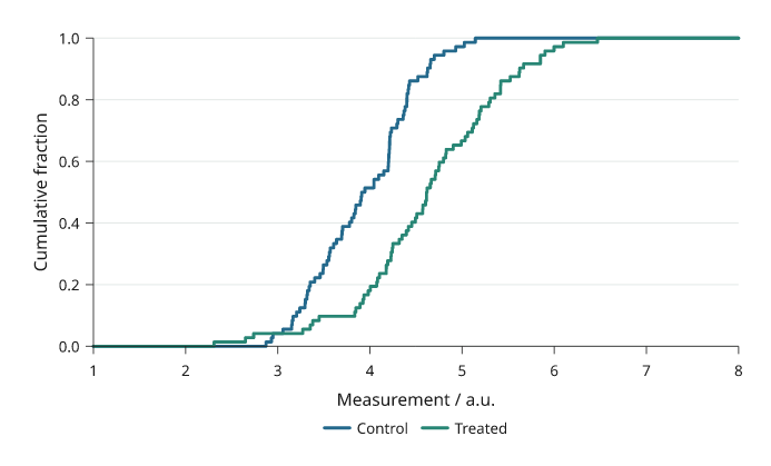
Rendered from the code above, with the same 72 observations per group used above. The curves run flat to both ends of the x axis.

Ridgelines¶

ridgeline draws one kernel density per category on a shared x scale, with the categories on a band y scale. Each ridge stands on the lower edge of its category's row, and overlap is the height of the tallest ridge in rows, so values above 1 let a ridge rise into the rows above it. Ridges are filled with an opaque colour and drawn from the top down, so lower ridges cover the ones behind them.

scale='shared' (default) uses one height scale for all ridges, so their areas compare; scale='each' gives every ridge the same peak height. By default all ridges are scaled down by one factor if the top ones would rise above the plot area, so overlap is a maximum; fit=False keeps it and lets them rise above. The bandwidth follows the same rule as violin.

import inklet as i
import random

rng = random.Random(403)
stages = ['E12', 'E14', 'E16', 'E18', 'P0', 'P7']
onsets = {s: [rng.gauss(2 + k * .9, .9 - .08 * k) for _ in range(80)]
          + [rng.gauss(4.2 + k * .9, .4) for _ in range(20 * (k % 3))]
          for k, s in enumerate(stages)}
p = i.plot_spec(x=(0, 10), y=stages[::-1], height=48)
p.ridgeline(onsets, overlap=1.8,
            color=['#24698c', '#2d7d8a', '#3a9083', '#5aa374', '#8bb35f', '#c2bf52'],
            stroke='white', stroke_width=.3)
p.axes(x='Onset time / h')
doc = i.document(width=90)
doc.add('ridgeline', p)
doc.save('ridgeline.svg', 'ridgeline.pdf')

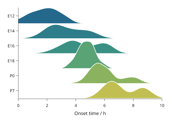
Rendered from the code above. Each ridge is a kernel density of 80 to 120 simulated onset times; heights share one scale.

Rainclouds¶

raincloud draws, for each group, a half violin, a narrow box and every observation. It takes the same groups as violin and swarm. Each group's slot is split into three lanes: the half violin stands on the category's centre line, the box sits just beside it, and the observations fill the far half of the slot. With orient='h' (default) the groups are on the y axis and the half violin rises up the page; with orient='v' it extends to the right.

The half violin uses the violin bandwidth rule. The box shows the quartiles, the median and whiskers to the furthest observations within 1.5 interquartile ranges, without caps; outliers are not drawn separately because every observation is shown. points='jitter' (default) moves each observation sideways by a random offset from a generator seeded by seed, so the figure is the same on every run. points='swarm' packs them as swarm does, and points=None leaves them out. box=False leaves out the box. The points use each group's colour and the half violin a paler blend of it.

import inklet as i
import random

rng = random.Random(402)
samples = {'Control': [rng.gauss(4.1, .62) for _ in range(72)],
           'Treated': [rng.gauss(4.65, .78) for _ in range(52)]
           + [rng.gauss(6.2, .3) for _ in range(20)]}
p = i.plot_spec(x=(1, 8), y=['Treated', 'Control'], height=44)
p.raincloud(samples, color=['#24698c', '#288675'], size=.9)
p.axes(x='Measurement / a.u.')
doc = i.document(width=90)
doc.add('raincloud', p)
doc.save('raincloud.svg', 'raincloud.pdf')

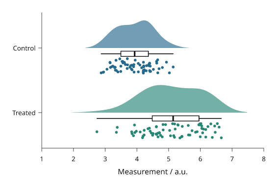
Rendered from the code above. The treated group has a second mode near 6, which the half violin and the points show and the box does not.

Survival curves¶

kaplan_meier draws Kaplan–Meier survival curves. Pass a mapping of group name to (durations, events), where events is true for an observed event and false for a censored subject. Each curve is a step line from 1 at time 0 to the last observed time. A short vertical tick marks each censoring time.

The estimate is the product-limit estimate with Greenwood's variance. The shaded band is a 95% log-log confidence interval, which stays between 0 and 1. band='linear' gives the plain Greenwood interval, and band=None leaves the band out. inklet.plot.kaplan_meier(durations, events) returns the estimate without drawing it: times, survival, numbers at risk, variance, band and median.

at_risk() adds the number-at-risk table below everything already drawn, so call it after axes(). Each column sits under an x tick, and each row is set in its curve's colour. Inklet does not run a log-rank test. To annotate a p-value computed elsewhere, pass pvalue=.

import inklet as i
import random

rng = random.Random(7)

def arm(rate, n=60):
    durations, events = [], []
    for _ in range(n):
        event, dropout = rng.expovariate(rate), rng.uniform(6, 60)
        durations.append(round(min(event, dropout, 36), 1))
        events.append(event <= min(dropout, 36))
    return durations, events

p = i.panel(62, 38, x=(0, 36), y=(0, 1))
p.kaplan_meier({'Control': arm(1 / 14), 'Treated': arm(1 / 30)},
               color=['#262626', '#24698c'], pvalue=0.003)
p.axes(x='Time / months', y='Survival probability',
       x_options={'ticks': [0, 6, 12, 18, 24, 30, 36]})
p.legend(corner='ne')
p.at_risk(ticks=[0, 6, 12, 18, 24, 30, 36])
fig = i.figure(width=90)
fig.add(p.build())
fig.save('survival.svg', 'survival.pdf')

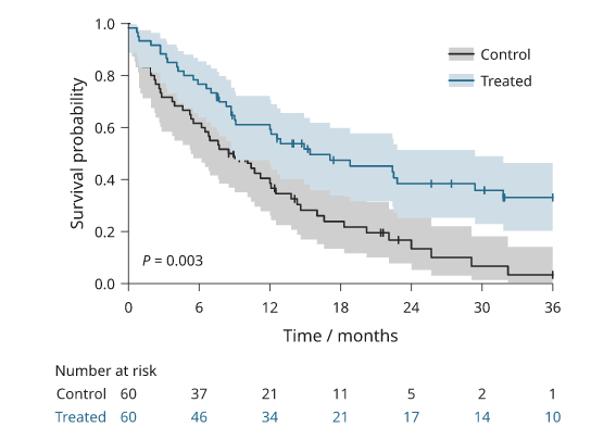
Rendered from the code above with simulated follow-up of 60 subjects per group. The p-value is illustrative and was not computed from these data.

Split violins¶

split_violin compares two conditions per category: the first is the left half of each violin and the second the right half (with orient='h', the upper and lower halves). The groups are spelled as for violin, and each half is the violin kernel density with the same bandwidth rule, cut and samples. By default both halves of a category share one width scale, so their areas are equal; scale='each' gives each half the full width. median=True (default) draws each half's median as a solid line and quartiles=True its quartiles as dashed lines. name= puts both conditions in the legend.

import inklet as i
import random

rng = random.Random(404)
regions = ['CA1', 'CA3', 'DG']
control = {r: [rng.gauss(4 + 1.2 * k, .9) for _ in range(80)] for k, r in enumerate(regions)}
treated = {r: [rng.gauss(4.6 + .8 * k, 1.1) for _ in range(60)]
           + [rng.gauss(9, .5) for _ in range(12 + 6 * k)] for k, r in enumerate(regions)}
p = i.plot_spec(x=regions, y=(0, 12), height=44)
p.split_violin(control, treated, name=['Control', 'Treated'], quartiles=True,
               color=['#e6b93f', '#9cc3d5'])
p.axes(y='Firing rate / Hz').legend(side='top')
doc = i.document(width=90)
doc.add('split-violin', p)
doc.save('split-violin.svg', 'split-violin.pdf')

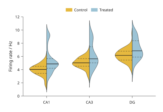
Simulated data. The treated half shows a second mode near 9 Hz.

Significance brackets¶

brackets draws many significance brackets in one call. It takes a list of (group_a, group_b, value), where the value is a p-value or the text to write, and draws them with bracket, shortest span first. Each bracket clears the data between its ends and the brackets already drawn there, so nested comparisons stack upward and a short one sits just over its own data.

format='stars' (default) writes ****, ***, ** or * for p below 0.0001, 0.001, 0.01 and 0.05, and ns otherwise; format='p' writes "P = 0.004" or "P < 0.001". hide_ns=True leaves out comparisons that are not significant. No test is run: the p-values are yours. inklet.plot.format_p formats one p-value.

import inklet as i
import random

rng = random.Random(405)
genotypes = ['wt', 'het', 'ko', 'rescue']
response = {g: [rng.gauss(m, .45) for _ in range(10)]
            for g, m in zip(genotypes, (3.0, 3.4, 5.0, 3.6))}
p = i.plot_spec(x=genotypes, y=(0, 10), height=44)
p.boxplot(response, outliers=False)
p.swarm(response, color=['#24698c'] * 4)
p.brackets([('wt', 'het', .21), ('wt', 'ko', 2e-5), ('het', 'ko', .004),
            ('ko', 'rescue', 7e-4), ('wt', 'rescue', .031)])
p.axes(y='Response / a.u.')
doc = i.document(width=80)
doc.add('brackets', p)
doc.save('brackets.svg', 'brackets.pdf')

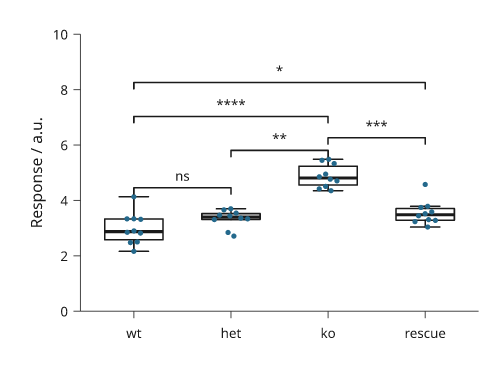
Simulated data with made-up p-values.

Histogram outlines, groups and cumulative counts¶

hist takes a mapping of group name to values and bins every group on the same edges, taken from all the groups together, so the bars line up and the heights compare. Groups are drawn as translucent filled outlines in the ink palette and named for legend(). histtype='step' draws the outline alone, 'stepfilled' fills it without edges between bins, and the default for one sample stays touching bars. cumulative=True draws running totals; with density=True they end at one, the empirical distribution function on the bins' upper edges.

import inklet as i
import random
rng = random.Random(406)
groups = {'Control': [rng.gauss(4.0, .8) for _ in range(240)],
          'Treated': [rng.gauss(5.1, 1.1) for _ in range(180)]}
counts = i.plot_spec(x=(0, 9), y=(0, 60), height=40)
counts.hist(groups, 24)
counts.axes(x='Response / a.u.', y='Count')
counts.legend(corner='ne')
running = i.plot_spec(x=(0, 9), y=(0, 1), height=40)
running.hist(groups, 40, density=True, cumulative=True, histtype='step')
running.axes(x='Response / a.u.', y='Cumulative fraction')
doc = i.document(width=120, columns=[1, 1], gap=8)
doc.add('counts', counts, row=0, column=0)
doc.add('running', running, row=0, column=1)
doc.save('hist-groups.svg', 'hist-groups.pdf')

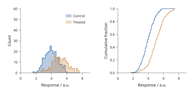
Rendered from the code above. Both groups share one set of bin edges; the right panel shows the fraction of each group at or below each bin's upper edge.

Kernel density curves¶

kde draws a Gaussian kernel density of one sample or of each group in a mapping, in stdlib Python. bandwidth='scott' (default) is R's bw.nrd, 1.06 min(sd, IQR/1.34) n^-1/5; 'silverman' is bw.nrd0, with 0.9 in place of 1.06; a number sets it in data units, and adjust scales any of them. fill=True shades under each curve at 25% opacity so groups stay visible through each other. stat='count' multiplies by the sample size, so the areas compare group sizes. On a log axis the density is estimated in log units. inklet.plot.kde_curve returns the curve without drawing it. The bandwidth is a smoothing choice; report it with the figure.

import inklet as i
import random
rng = random.Random(407)
groups = {'Control': [rng.gauss(4.0, .8) for _ in range(240)],
          'Treated': [rng.gauss(5.1, 1.1) for _ in range(180)]}
p = i.plot_spec(x=(0, 9), y=(0, .55), height=40)
p.kde(groups, fill=True)
p.axes(x='Response / a.u.', y='Density')
p.legend(corner='ne')
doc = i.document(width=80)
doc.add('kde', p)
doc.save('kde.svg', 'kde.pdf')

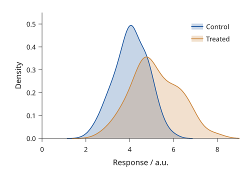
Rendered from the code above, with Scott's rule chosen separately for each group.

Letter-value plots¶

A box plot of 5,000 observations marks hundreds of ordinary tail values as outliers. boxen (a letter-value plot) keeps going out into the tails: the inner box spans the quartiles, the next the eighths, then the sixteenths, each narrower and paler than the one inside. depth='tukey' (default) draws floor(log2 n) - 3 boxes; 'trustworthy' draws as many as have non-overlapping 95% intervals. The median is a paper-coloured line. Values beyond the outermost box are dots. inklet.plot.letter_values returns the boxes.

import inklet as i
import random
rng = random.Random(408)
samples = {'Normal': [rng.gauss(0, 1) for _ in range(5000)],
           'Wide': [rng.gauss(.5, 1.6) for _ in range(5000)],
           'Skewed': [rng.expovariate(1) - 1 for _ in range(5000)]}
p = i.plot_spec(x=list(samples), y=(-7, 9), height=44)
p.boxen(samples)
p.axes(y='Value / a.u.')
doc = i.document(width=80)
doc.add('boxen', p)
doc.save('boxen.svg', 'boxen.pdf')

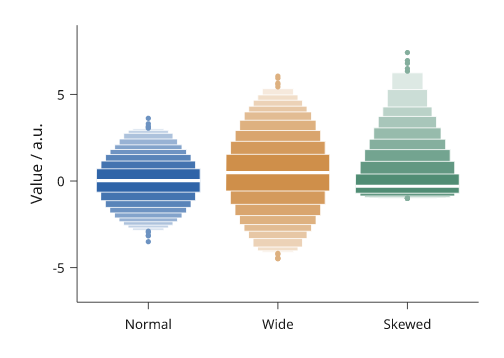
Rendered from the code above: 5,000 simulated values per group, seven letter values each.

Strip and sina plots¶

strip draws every observation, jittered across its group's slot by a seeded random generator: the same call draws the same figure, and seed= changes the draw. Over boxplot(..., outliers=False) it shows the summary and the points together. sina spreads each point by at most the group's kernel density at its value, so the points take a violin's outline and every value stays visible. Only the sideways position is random; values are exact.

import inklet as i
import random
rng = random.Random(409)
small = {'wt': [rng.gauss(3.0, .5) for _ in range(40)],
         'ko': [rng.gauss(4.2, .8) for _ in range(40)]}
large = {'wt': [rng.gauss(3.0, .5) for _ in range(400)],
         'ko': [rng.gauss(4.2, .8) + (1.2 if rng.random() < .3 else 0)
                for _ in range(400)]}
strip = i.plot_spec(x=['wt', 'ko'], y=(0, 8), height=44)
strip.boxplot(small, outliers=False)
strip.strip(small, size=.8)
strip.axes(y='Response / a.u.')
sina = i.plot_spec(x=['wt', 'ko'], y=(0, 8), height=44)
sina.sina(large, size=.6)
sina.axes(y='Response / a.u.')
doc = i.document(width=100, columns=[1, 1], gap=8)
doc.add('strip', strip, row=0, column=0)
doc.add('sina', sina, row=0, column=1)
doc.save('strip-sina.svg', 'strip-sina.pdf')

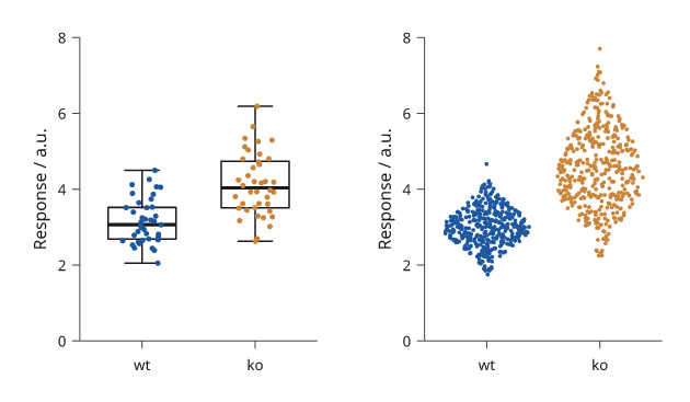
Rendered from the code above. Left, 40 observations per group over their boxes; right, 400 per group spread by their densities.

Quantile-quantile and probability plots¶

qq plots each sorted value against the standard normal quantile at its plotting position (R's ppoints), with a reference line through the first and third quartiles, as R's qqline draws. A normal sample follows the line; heavy tails bend away from it at both ends. line='fit' uses the mean and standard deviation instead. pp plots the fitted normal CDF against the empirical probabilities, with the diagonal. A PP plot is most sensitive in the middle of the distribution, a QQ plot in the tails. dist= takes another statistics.NormalDist or any quantile function (for pp, any CDF).

import inklet as i
import random
rng = random.Random(410)
heavy = [rng.gauss(0, 1) / max(.25, abs(rng.gauss(0, 1))) ** .5
         for _ in range(150)]
qq = i.plot_spec(x=(-3, 3), y=(-6, 6), height=40)
qq.qq(heavy)
qq.axes(x='Normal quantile', y='Sample quantile')
pp = i.plot_spec(x=(0, 1), y=(0, 1), height=40)
pp.pp(heavy)
pp.axes(x='Normal probability', y='Empirical probability')
doc = i.document(width=100, columns=[1, 1], gap=8)
doc.add('qq', qq, row=0, column=0)
doc.add('pp', pp, row=0, column=1)
doc.save('qq.svg', 'qq.pdf')

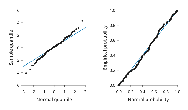
Rendered from the code above. The sample is heavy-tailed by construction, so its extreme values bend away from the QQ reference line.

Next steps¶

Relationships between variables covers 2D densities, regression, agreement plots and pair plots.

Compare plot types, configure axes and scales, or arrange several panels. For exact options, see the API.