Genomics and ternary plots¶

Three specialist plots: the Manhattan plot of a genome-wide association study, the MA plot of a differential-expression test, and the ternary plot of three-part compositions. For the volcano plot, see Lines and points.

Manhattan plots¶

inklet.manhattan(chromosome, position, p) returns a panel with its axes, ready for more layers or for fig.add. Chromosomes are laid end to end in natural order (1, 2, ..., 10, ..., X, Y, MT; a chr prefix is fine), or in order=. Points alternate between two shades per chromosome, and bands=True also shades every other chromosome's span.

threshold draws the genome-wide significance line (5e-8, red) and suggestive a grey one (1e-5); either can be None. With labels=, the top lead hits are named: a lead hit is the variant below threshold with the smallest p within window base pairs (1 Mb). highlight= draws chosen variants in red. For a million variants, pass raster=True to rasterise the points.

inklet.plot.manhattan_layout returns the same positions, chromosome spans and lead hits without drawing anything.

import inklet as i
import math
import random

rng = random.Random(11)
peaks = {'2': (60e6, 14), '6': (32e6, 22), '11': (100e6, 9), '16': (50e6, 10.5)}
chrom, pos, pvalues, ids = [], [], [], []
for number in list(range(1, 23)) + ['X']:
    c = str(number)
    length = 155e6 if c == 'X' else 250e6 * (1 - 0.035 * (int(c) - 1))
    for k in range(int(length / 2e6)):
        x = rng.uniform(0, length)
        y = rng.expovariate(1.0)
        if c in peaks and abs(x - peaks[c][0]) < 3e6:
            y = max(y, peaks[c][1] * math.exp(-((x - peaks[c][0]) / 1e6) ** 2))
        chrom.append('chr' + c); pos.append(x); pvalues.append(10 ** -y)
        ids.append(f'rs{rng.randint(1000, 999999)}')
    if c in peaks:
        for _ in range(30):
            x = peaks[c][0] + rng.gauss(0, 0.6e6)
            y = peaks[c][1] * math.exp(-((x - peaks[c][0]) / 1e6) ** 2) + rng.uniform(0, 1)
            chrom.append('chr' + c); pos.append(x); pvalues.append(10 ** -y)
            ids.append(f'rs{rng.randint(1000, 999999)}')
gwas = i.manhattan(chrom, pos, pvalues, labels=ids, top=4, width=150, height=40)
fig = i.figure(width=170)
fig.add(gwas.build())
fig.save('manhattan.svg', 'manhattan.pdf')

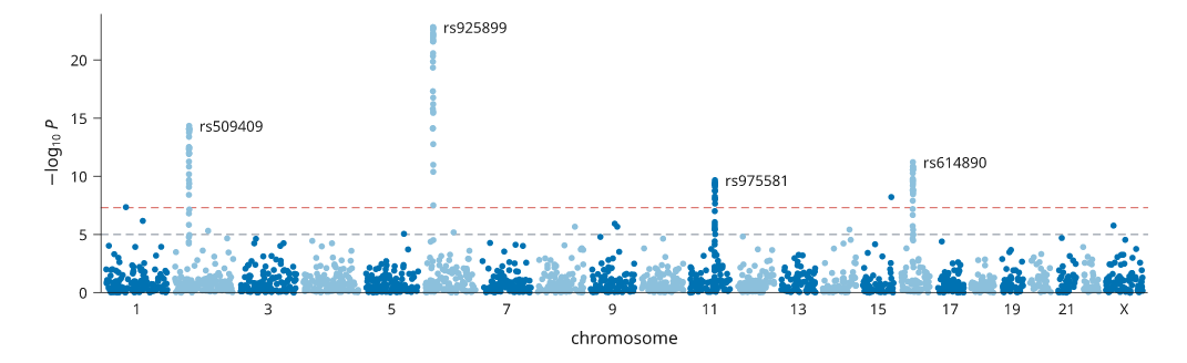
Simulated association results with four loci above genome-wide significance.

MA plots¶

Panel.ma(mean, fold, p) plots each feature's log2 fold change against its mean expression. The mean is drawn as log2(mean + 1) unless log=False. Points are classified as volcano classifies them: "up" and "down" need p below p_threshold and |fold| of at least fold_threshold. Without p, fold change alone decides. Non-significant points are pale grey and drawn first, and a hairline marks a fold change of 0. labels= names the top most significant points.

import inklet as i
import math
import random

rng = random.Random(4)
mean = [2 ** rng.uniform(0, 15) for _ in range(1500)]
fold = [rng.gauss(0, 0.5) + (rng.random() < 0.05) * rng.choice([-1, 1]) * rng.uniform(1, 4)
        for _ in range(1500)]
padj = [min(1.0, 2 * math.exp(-abs(f) * 4 * rng.uniform(0.2, 1.5))) for f in fold]
genes = [f'Gene{k}' for k in range(1500)]
ma = i.panel(55, 40, x=(0, 16), y=(-6, 6))
ma.ma(mean, fold, padj, labels=genes, top=5, name=['down', None, 'up'])
ma.axes(x='log_{2} mean expression', y='log_{2} fold change').legend(side='right')
fig = i.figure(width=89)
fig.add(ma.build())
fig.save('ma.svg', 'ma.pdf')

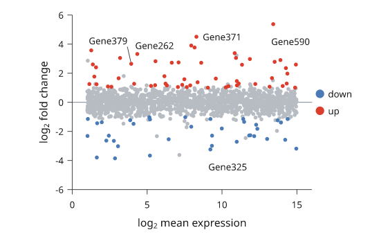
Simulated expression. About one gene in twenty is differentially expressed.

Ternary plots¶

Panel.ternary(points) draws three-part compositions in an equilateral triangle fitted into the plot area. Each (a, b, c) point is normalised to fractions of its sum. The first call draws the triangle with labels[0] at the top vertex, labels[1] bottom left and labels[2] bottom right, a pale grid and tick labels as parts of total (100). Later calls add points to the same triangle. The points are an ordinary scatter, so name=, color=, size= and ramps work, and legend() names the series.

import inklet as i
import random

rng = random.Random(2)
upland = [(rng.uniform(5, 30), rng.uniform(40, 80), rng.uniform(10, 30)) for _ in range(30)]
valley = [(rng.uniform(30, 60), rng.uniform(5, 25), rng.uniform(25, 50)) for _ in range(30)]
soil = i.panel(50, 45)
soil.ternary(upland, labels=('clay', 'sand', 'silt'), name='upland')
soil.ternary(valley, name='valley').legend(side='right')
fig = i.figure(width=80)
fig.add(soil.build())
fig.save('ternary.svg', 'ternary.pdf')

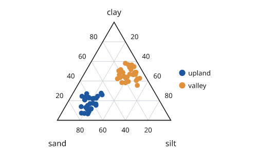
Illustrative soil samples. Upland soils are sandy and valley soils richer in clay and silt.

Next steps¶

Compare plot types, see volcano plots, or arrange several panels. For exact options, see the API.