How do I…¶

Short answers to the questions people ask most, each with a complete snippet for the one-call API described in Charts in one call. The snippets run as written, and each figure they draw lints clean.

Draw a correlation matrix with a centred colour scale¶

Pass a diverging palette, center=0 and colorbar_title= to i.heatmap.

import inklet as i

genes = ['A', 'B', 'C', 'D']
r = [
    [1.00, 0.62, -0.31, 0.08],
    [0.62, 1.00, -0.45, 0.12],
    [-0.31, -0.45, 1.00, -0.70],
    [0.08, 0.12, -0.70, 1.00],
]
chart = i.heatmap(r, x=genes, y=genes, palette='RdBu', center=0, colorbar_title='r')
chart.save('correlation.pdf')

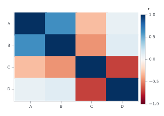
center=0 puts the neutral colour at zero, so positive and negative values get equal weight. Without it the scale runs from the smallest value to the largest. The first row is drawn at the top.

Plot two quantities in different units on one chart¶

Name the series in secondary_y=, and it is drawn against a right-hand axis titled with its column.

import inklet as i

table = {
    'month': ['Jan', 'Feb', 'Mar', 'Apr', 'May', 'Jun'],
    'rain (mm)': [62, 48, 55, 41, 38, 30],
    'temp (°C)': [4.1, 5.0, 8.2, 12.5, 16.9, 20.3],
}
chart = i.bar(table, x='month', y='rain (mm)')
chart.line(table, x='month', y='temp (°C)', secondary_y='temp (°C)')
chart.labels(x='Month', y='Rain / mm', y2='Mean temperature / °C')
chart.save('rain-temperature.pdf')

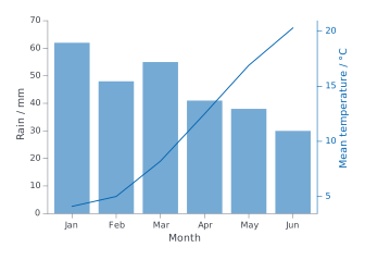
A second y scale invites misreading: the two lines can cross, or look alike, for no reason in the data. Two panels that share an x axis are often clearer. Stack them with /, as in i.line(...) / i.bar(...). Use secondary_y= when the quantities must share one x axis, as they do here. chart.twin_y() is refused on a quick chart; secondary_y= replaces it.

Label only the top N points of a scatter¶

Give text= a column that holds a label for the points you want and None for the others. Rows with no label get no label and no leader line.

import inklet as i

table = {
    'gene': ['Tnf', 'Il6', 'Cxcl10', 'Nos2', 'Ifit1', 'Actb', 'Gapdh', 'Myc'],
    'fold': [2.6, -3.4, 4.1, 3.5, -5.1, 0.1, -0.2, 1.2],
    'signal': [7.1, 6.8, 8.2, 6.0, 7.9, 9.5, 9.7, 5.4],
}
# The three genes with the largest fold change, up or down.
n = 3
biggest = sorted(range(len(table['gene'])), key=lambda k: abs(table['fold'][k]), reverse=True)[:n]
table['label'] = [gene if k in biggest else None for k, gene in enumerate(table['gene'])]

chart = i.scatter(table, x='fold', y='signal', text='label')
chart.save('top-genes.pdf')

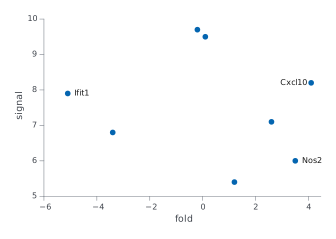
With pandas, the same column is one line: df['label'] = df['gene'].where(df['fold'].abs().rank(ascending=False) <= 3). Missing values count as None.

Show means with SEM error bars and the raw points¶

Use agg='mean', error_y='sem' and points=True on i.bar.

import inklet as i

table = {
    'group': ['control'] * 8 + ['low dose'] * 8 + ['high dose'] * 8,
    'response': [
        1.12, 0.67, 1.45, 1.05, 0.92, 1.66, 1.36, 0.91,
        1.41, 1.62, 1.07, 1.28, 1.79, 1.38, 1.65, 1.06,
        1.61, 2.10, 2.01, 1.99, 1.64, 1.56, 1.63, 1.52,
    ],
}
chart = i.bar(table, x='group', y='response', agg='mean', error_y='sem', points=True)
chart.save('response.pdf')

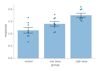
Without agg=, bar sums the rows that share a category. Eight measurements per group would draw a bar about eight times the mean, so lint reports ROWS_COMBINED for any category with more than one row. Pass agg='sum' when the rows really are parts of a total. error_y also takes 'sd' and 'ci95'.

Draw horizontal bars¶

Pass orient='h'. The category column (x=) runs down the left, and the values (y=) run along the bottom. The first row is at the top, so the chart reads down the table in the order it was written.

import inklet as i

table = {
    'pathway': ['Autophagy', 'Apoptosis', 'Cell cycle', 'Glycolysis'],
    'score': [0.9, 1.7, 2.4, 3.1],
}
chart = i.bar(table, x='pathway', y='score', orient='h',
              xlabel='Enrichment score', ylabel='Pathway')
chart.save('pathways.pdf')

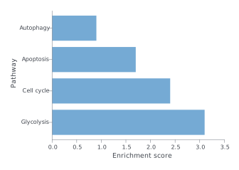
xlabel always titles the horizontal axis and ylabel the vertical one, whatever the orientation. So with orient='h' the value name goes in xlabel. Without them, the column names are used, and they land on the same axes.

Add a labelled reference line¶

Call chart.hline(y, label=...) or chart.vline(x, label=...). The label is placed clear of the data. If it crowds the data, give the plot headroom with ylim= and keep the label to one side with label_side=: 'n' or 's' for an hline, 'e' or 'w' for a vline.

import inklet as i

table = {
    'dose': [1, 2, 3, 4, 5, 6, 7, 8],
    'response': [2.1, 3.9, 6.2, 7.8, 8.1, 9.5, 9.7, 9.9],
}
chart = i.scatter(table, x='dose', y='response', ylim=(0, 12))
chart.hline(5.0, label='half max', label_side='n')
chart.vline(4.0, label='EC50', label_side='e')
chart.save('reference-lines.pdf')

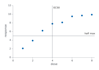
A labelled line is drawn in front of the data, so it shows even under a bar chart.

Write subscripts, superscripts and Greek in labels¶

Write _{...} for a subscript and ^{...} for a superscript. Type Greek letters as characters: α, β, µ. Matplotlib's $...$ mathtext is not read. It prints as typed, dollar signs and backslashes included, so $\alpha$ shows as written.

import inklet as i

table = {'dose': [1, 2, 4, 8, 16], 'uptake': [1.2, 2.1, 3.4, 3.9, 4.0]}
chart = i.scatter(
    table, x='dose', y='uptake',
    title='CO_{2} uptake, α = 0.05',
    xlabel='Dose / mg kg^{-1}',
    ylabel='Uptake / µmol m^{-2} s^{-1}',
)
chart.save('uptake.pdf')

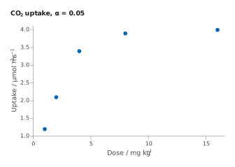
The same markup works in titles and axis labels. Other markup: **bold**, //italic// and {#c1121f|coloured}. A backslash makes a markup character literal, as in \_ or \{.

Typesetting symbols. Set variables in italic, and units, numbers, labels and chemical symbols upright, as a journal's style guide asks. For example, "//m//_{ν}^{2} (eV^{2})" sets mν² (eV²) and "//E//_{0} (eV)" sets E₀ (eV). The italic is a real italic face, so it is measured and wrapped like the rest of the label.

Alignment. The lines of a multi-line label are centred on one another by default, so a name over a value looks ragged. Pass align="start" for a flush left edge; "end" and "justify" (which needs width=) are also accepted. annotate() and text() take it, and a title built with inklet.text(..., align="start") keeps its lines flush left.

Mark significant differences between groups¶

Call chart.brackets([(a, b, p), ...]) on a chart with categories. Each triple is two group names and a p-value, drawn as stars by default. The p-values are yours: brackets runs no test. Leave headroom above the data with ylim=, so the stacked brackets fit inside the plot.

import inklet as i

table = {
    'group': ['control'] * 6 + ['low dose'] * 6 + ['high dose'] * 6,
    'value': [
        1.00, 1.10, 1.30, 1.20, 1.00, 1.40,
        0.90, 1.20, 1.50, 1.10, 1.30, 1.60,
        1.00, 1.00, 1.40, 1.30, 1.10, 1.20,
    ],
}
chart = i.boxplot(table, x='group', y='value', ylim=(0.5, 2.0))
chart.brackets([
    ('control', 'low dose', 0.03),
    ('control', 'high dose', 0.0004),
    ('low dose', 'high dose', 0.2),
])
chart.save('comparisons.pdf')

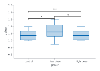
format='p' writes the P value instead of stars, and hide_ns=True leaves out the pairs that are not significant.

Label the panels of a figure¶

Do not put "a" or "b" in a title. A layout with | or / adds the letters a, b, c… in order, so a title with its own letter shows it twice. To turn the letters off, pass letters=False to the layout.

import inklet as i

control = i.line(x=[0, 1, 2, 3], y=[1.0, 1.2, 1.5, 1.6],
                 title='Control', xlabel='Time (h)', ylabel='Signal (a.u.)')
treated = i.line(x=[0, 1, 2, 3], y=[1.0, 1.8, 2.6, 3.1],
                 title='Treated', xlabel='Time (h)', ylabel='Signal (a.u.)')
figure = control | treated
figure.save('panels.pdf')

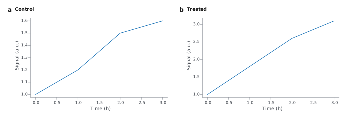
Without letters, the same figure is:

import inklet as i

control = i.line(x=[0, 1, 2, 3], y=[1.0, 1.2, 1.5, 1.6],
                 title='Control', xlabel='Time (h)', ylabel='Signal (a.u.)')
treated = i.line(x=[0, 1, 2, 3], y=[1.0, 1.8, 2.6, 3.1],
                 title='Treated', xlabel='Time (h)', ylabel='Signal (a.u.)')
figure = (control | treated).options(letters=False)
figure.save('panels-unlettered.pdf')

Layer, annotate and refine a chart¶

Chart methods change the chart in place and return it, so calls chain. Some are defined on Chart; the rest are the plot's own methods, forwarded from the chart to chart.spec. The call is the same either way.

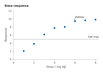
import inklet as i

table = {
    'dose': [1, 2, 3, 4, 5, 6, 7, 8],
    'response': [2.1, 3.9, 6.2, 7.8, 8.1, 9.5, 9.7, 9.9],
}
chart = (
    i.scatter(table, x='dose', y='response', ylim=(0, 12))
    .annotate(6, 9.5, 'plateau')
    .hline(5.0, label='half max', label_side='n')
    .labels(x='Dose / mg kg^{-1}', y='Response', title='Dose response')
    .size(width='single')
)
chart.save('chained.pdf')

Plot large data¶

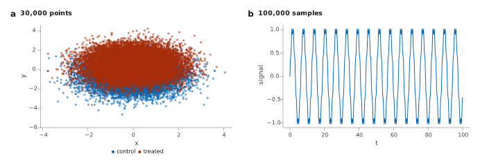
Nothing needs setting. A scatter panel with more than 20,000 points is drawn as one image of its markers, so the file stays small and the axes, labels and key stay vector. A line thins itself with simplify='auto', the default. It drops points that stay within 0.02 mm of the line through the kept points, which is invisible in print. Pass raster=False to keep every scatter point as vector, or simplify=None to keep every line point.

import math
import random
import inklet as i

rng = random.Random(7)
cloud = {'x': [], 'y': [], 'group': []}
for k in range(30_000):
    group = 'treated' if k % 2 else 'control'
    cloud['x'].append(rng.gauss(0, 1))
    cloud['y'].append(rng.gauss(0.5 if group == 'treated' else -0.5, 1))
    cloud['group'].append(group)

trace = {'t': [k * 0.001 for k in range(100_000)]}
trace['signal'] = [math.sin(t) + 0.1 * math.sin(7 * t) for t in trace['t']]

figure = (i.scatter(cloud, x='x', y='y', color='group', title='30,000 points')
          | i.line(trace, x='t', y='signal', title='100,000 samples'))
figure.save('large-data.pdf')

Save a figure for a journal¶

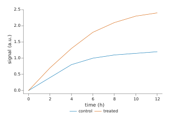
Pass width='single' (89 mm) or width='double' (183 mm), choose the journal's style preset, and save a PDF. Then check the figure before you submit it.

import inklet as i

table = {
    'time (h)': [0, 2, 4, 6, 8, 10, 12, 0, 2, 4, 6, 8, 10, 12],
    'signal (a.u.)': [0.0, 0.4, 0.8, 1.0, 1.1, 1.15, 1.2, 0.0, 0.7, 1.3, 1.8, 2.1, 2.3, 2.4],
    'condition': ['control'] * 7 + ['treated'] * 7,
}
chart = i.line(table, x='time (h)', y='signal (a.u.)', color='condition',
               width='single', style='scientific.nature')
chart.save('figure1.pdf')

save() writes the file and returns the compiled figure, whose report() lists overlapping or clipped text and type that is too small. From a shell, the same check runs on the script:

inklet check figure1.py --png preview.png

It prints the report and exits with 1 on errors. Add --strict to fail on warnings too. The script must leave its figure at module level, under the name chart or figure.