

On this page
Rebuild a journal figure
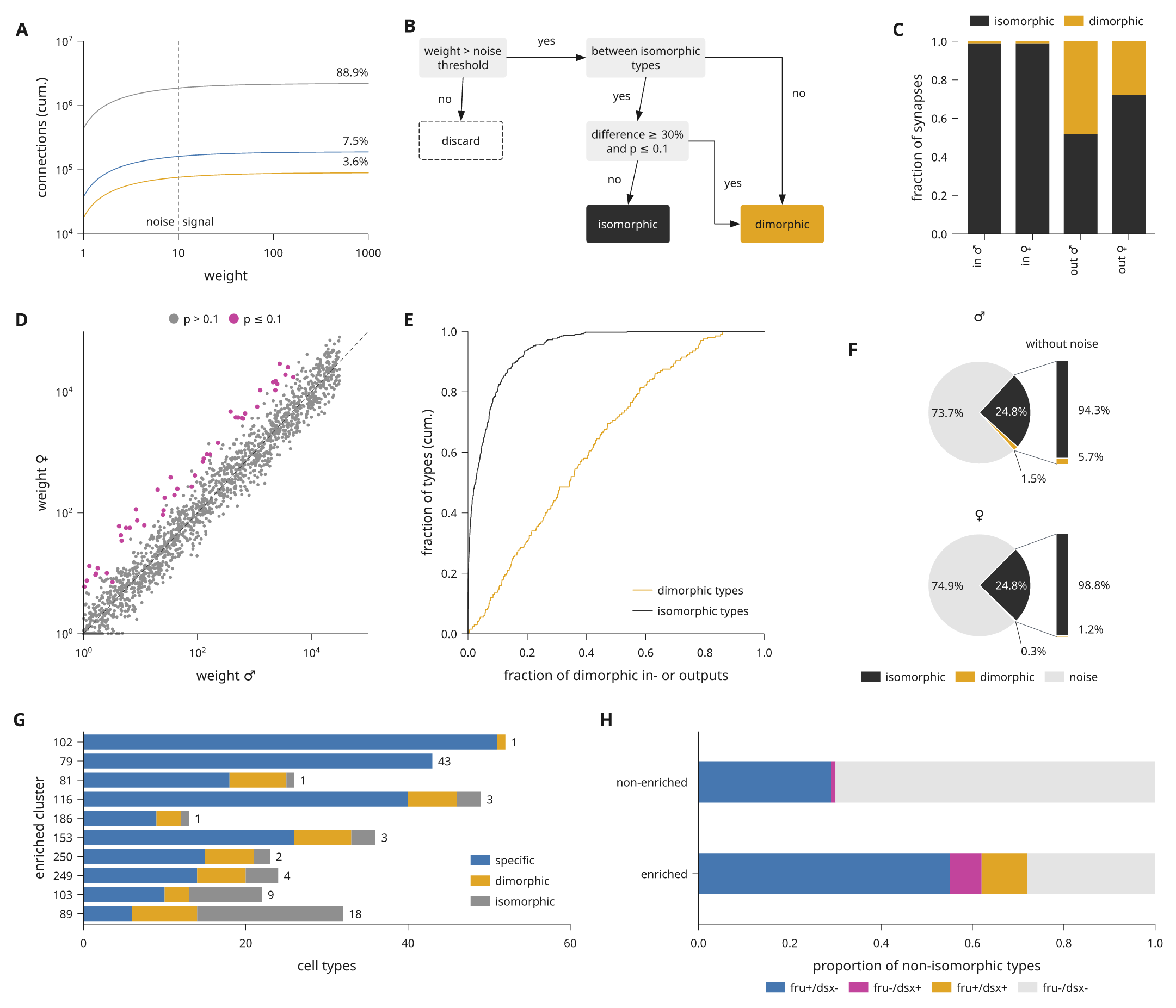
This page rebuilds a published figure page step by step. The model is a Cell figure on sexual dimorphism in a fly connectome. It has eight plot and diagram panels around its microscopy panels: cumulative counts on log axes, a decision flowchart, stacked fractions, a weight scatter, cumulative distributions, two pies with breakout bars, stacked bars with counts and proportion bars. The microscopy panels are left out. All data here are simulated or illustrative.
The complete script is
examples/journal_figure.py. The blocks below
are the same code, in the order the page is built. Each block runs after the
ones before it.
Read the page as a grid
Start by reading the original page as rows and columns. It is a 183 mm double column page with three rows of panels:
| Row | Panels | Columns of 12 |
|---|---|---|
| 1 | a counts, b flowchart, c fractions | 4, 5, 3 |
| 2 | d scatter, e distributions, f pies | 4, 4, 4 |
| 3 | g stacked bars, h proportion bars | 6, 6 |
Each panel becomes one item in a 12-column document. Row heights follow the
tallest panel in the row. With share_plot_margins=True the data areas in a
row share their top and bottom edges, whatever their tick labels.
Start from the preset
scientific.cell sets 6 pt text, 5 pt tick labels, bold panel letters and
0.25 pt hairlines, with a 183 mm page. The theme's palette gives the colours
that the panels share.
import math
import random

import inklet as i

style = i.preset('scientific.cell')
blue, amber, magenta, grey, green, ink = style.theme.palette
pale = '#e4e4e4'
rng = random.Random(5)
Row one: counts, flowchart and fractions
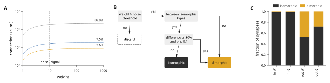
Panel a draws three cumulative curves on log axes. Each share is a text
anchored at the right end of its curve. A dashed vline marks the noise
threshold, with a short text on each side of it.
growth = i.plot_spec(height=30, x=i.log((1, 1000)), y=i.log((1e4, 1e7)))
for total, share, color in [(2.2e6, '88.9%', grey), (1.9e5, '7.5%', blue), (9e4, '3.6%', amber)]:
    curve = [(10 ** (t / 20), total * (1 - .8 * math.exp(-t / 12))) for t in range(61)]
    growth.line(curve, stroke=color)
    growth.text(1000, total, share, anchor='se', offset=(0, -.6))
growth.vline(10, stroke=ink, stroke_dash=(.5, .5), stroke_width=style.theme.hairline)
growth.text(10, 1.2e4, 'noise', anchor='se', offset=(-.6, 0))
growth.text(10, 1.2e4, 'signal', anchor='sw', offset=(.6, 0))
growth.axes(x='weight', y='connections (cum.)')
Panel b is a diagram, not a plot. A composition places measured modules in
millimetres, and each link names its ports. route='orthogonal' draws the two
links into the result box with right angles. See
measured connections for ports and routes.
def flowchart():
    scene = i.composition(64, 34)
    words = {'size': i.pt(5)}
    grey_box = {'fill': '#eeeeee', 'stroke': 'none', 'corner_radius': .5}
    steps = [('weight', 'weight > noise\nthreshold', 0, 0, grey_box, words),
             ('between', 'between isomorphic\ntypes', 26, 0, grey_box, words),
             ('test', 'difference ≥ 30%\nand p ≤ 0.1', 26, 13, grey_box, words),
             ('discard', 'discard', 0, 13,
              {'fill': 'none', 'stroke': ink, 'stroke_dash': (.6, .4), 'corner_radius': .5}, words),
             ('iso', 'isomorphic', 26, 26, {'fill': ink, 'stroke': 'none', 'corner_radius': .5},
              dict(words, text_fill='#ffffff')),
             ('dimo', 'dimorphic', 50, 26, {'fill': amber, 'stroke': 'none', 'corner_radius': .5},
              words)]
    for name, label, x, y, look, text in steps:
        scene.add(name, i.module(label, min_width=13, min_height=6, pad=.8,
                                 text_style=text, box_style=look), x=x, y=y)
    scene.link('weight:out', 'between:in', label='yes')
    scene.link('weight:s', 'discard:n', label='no')
    scene.link('between:s', 'test:n', label='yes')
    scene.link('between:out', 'dimo:n', label='no', route='orthogonal')
    scene.link('test:s', 'iso:n', label='no')
    scene.link('test:out', 'dimo:in', label='yes', route='orthogonal')
    return scene
Panel c stacks two fractions per group. The legend goes above the bars, and the group names are turned upright as in the original.
groups = ['in ♂', 'in ♀', 'out ♂', 'out ♀']
fractions = i.plot_spec(height=30, x=groups, y=(0, 1))
fractions.bars(groups, [[.99, .99, .52, .72], [.01, .01, .48, .28]], stacked=True,
               color=[ink, amber], name=['isomorphic', 'dimorphic'], width=.7)
fractions.axes(y='fraction of synapses', x_options={'rotate': 90})
fractions.legend(side='top')
Place the three panels to check the first row. Spans are 4, 5 and 3 columns.
align='nw' keeps the flowchart at its drawn size in the top left of its
cell.
row_one = style.document(columns=12, share_plot_margins=True).letters()
row_one.add('growth', growth, row=0, column=0, colspan=4)
row_one.add('flowchart', flowchart(), row=0, column=4, colspan=5, align='nw')
row_one.add('fractions', fractions, row=0, column=9, colspan=3)
Row two: scatter, distributions and pies
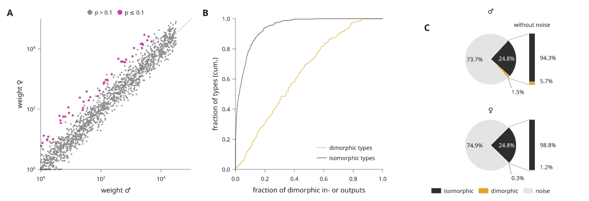
Panel d compares weights on two log axes. The dimorphic pairs are drawn over the rest, and a dashed diagonal marks equal weights.
pairs = []
for _ in range(1500):
    male = 10 ** rng.uniform(0, 4.5)
    pairs.append((male, max(1., male * 10 ** rng.gauss(0, .25))))
dimorphic = [(m, f * 6) for m, f in pairs[:60] if f * 6 < 3e4]
weights = i.plot_spec(height=30, x=i.log((1, 1e5)), y=i.log((1, 1e5)))
weights.scatter(pairs, size=.5, color=grey, name='p > 0.1')
weights.scatter(dimorphic, size=.7, color=magenta, name='p ≤ 0.1')
weights.line([(1, 1), (1e5, 1e5)], stroke=ink, stroke_dash=(.6, .5),
             stroke_width=style.theme.hairline)
weights.axes(x='weight ♂', y='weight ♀')
weights.legend()
Panel e is two cumulative distributions; ecdf sorts the samples and steps
through them. See cumulative distributions.
shares = i.plot_spec(height=30, x=(0, 1), y=(0, 1))
shares.ecdf([rng.betavariate(1.3, 2.5) for _ in range(200)], name='dimorphic types', stroke=amber)
shares.ecdf([rng.betavariate(.35, 6) for _ in range(400)], name='isomorphic types', stroke=ink)
shares.axes(x='fraction of dimorphic in- or outputs', y='fraction of types (cum.)')
shares.legend(corner='se')
Panel f is two small pies, one per sex. breakout turns each pie so that the
two signal slices face a bar that shows them without the noise slice. A slice
label that does not fit inside its slice moves outside the rim, onto a short
leader when it has to leave its slice. See
pie breakout bars.
def pies():
    rows = []
    for sex, iso, dimo, noise in [('♂', 24.8, 1.5, 73.7), ('♀', 24.8, .3, 74.9)]:
        p = i.polar(8)
        p.pie([iso, dimo, noise], color=[ink, amber, pale],
              labels=[f'{iso}%', f'{dimo}%', f'{noise}%'],
              name=['isomorphic', 'dimorphic', 'noise'] if sex == '♀' else None)
        p.breakout([0, 1], labels='{share:.1%}', gap=4,
                   title='without noise' if sex == '♂' else None)
        p.title(sex)
        if sex == '♀':
            p.legend(side='bottom', columns=3)
        rows.append(p.build())
    return i.column(rows, gap=3, align='left')
A polar panel is built at a fixed radius, so the pies go in as a component that is built when the page is compiled.
row_two = style.document(columns=12, share_plot_margins=True).letters()
row_two.add('weights', weights, row=0, column=0, colspan=4)
row_two.add('shares', shares, row=0, column=4, colspan=4)
row_two.add('pies', i.component(pies), row=0, column=8, colspan=4, align='n')
Row three: bars with counts and proportions
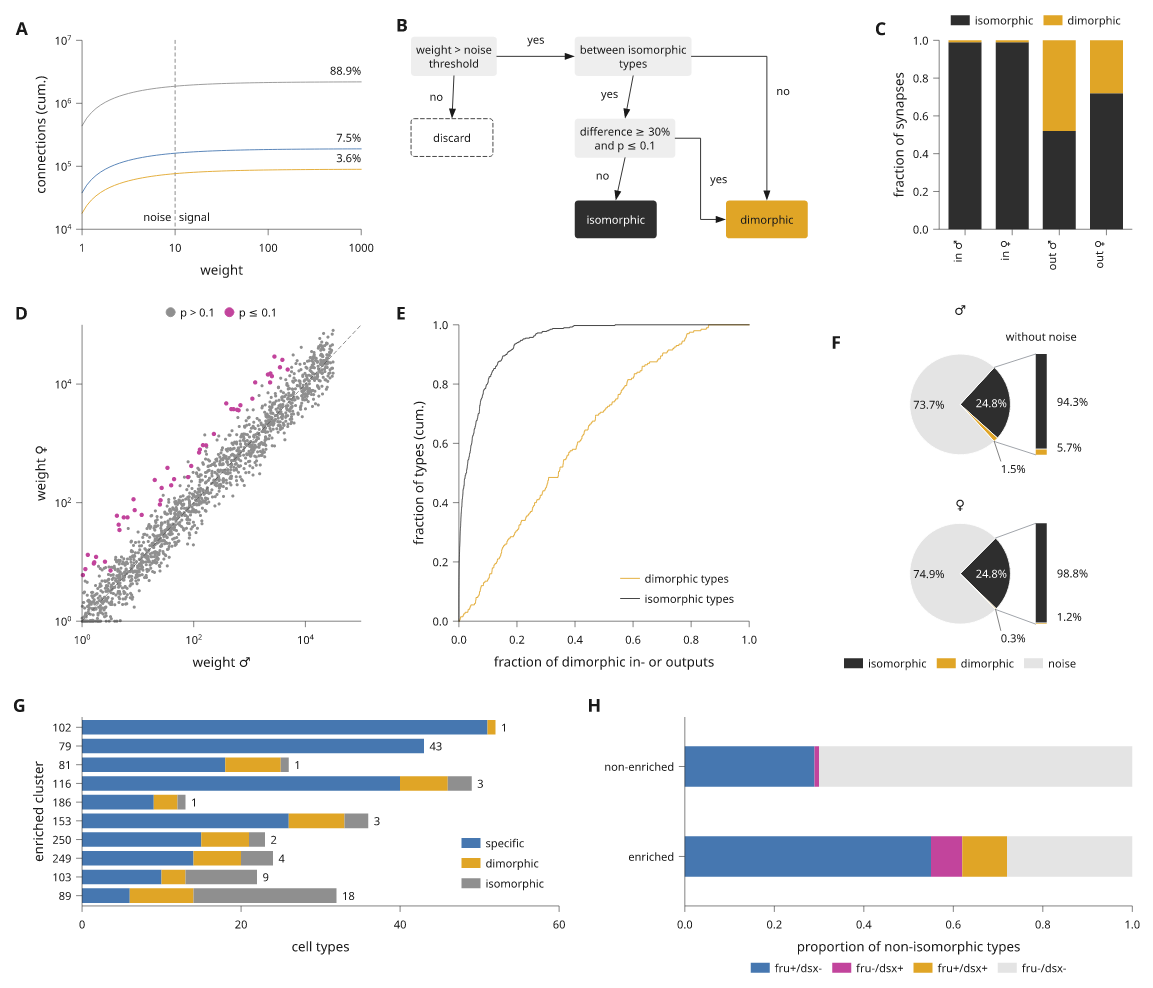
Panel g stacks three counts per cluster. labels=True writes each segment's
count where it fits, and the last segment's count at the free end of the bar.
See bar value labels.
clusters = ['102', '79', '81', '116', '186', '153', '250', '249', '103', '89']
specific = [51, 43, 18, 40, 9, 26, 15, 14, 10, 6]
dimorphic_types = [1, 0, 7, 6, 3, 7, 6, 6, 3, 8]
isomorphic = [0, 0, 1, 3, 1, 3, 2, 4, 9, 18]
counts = i.plot_spec(height=30, x=(0, 60), y=clusters[::-1])
counts.bars(clusters, [specific, dimorphic_types, isomorphic], stacked=True, orient='h',
            width=.78, color=[blue, amber, grey], name=['specific', 'dimorphic', 'isomorphic'],
            labels=True, stroke='none')
counts.axes(x='cell types', y='enriched cluster')
counts.legend()
Panel h shows proportions as two stacked horizontal bars, with a legend in four columns under the axis.
kinds = ['fru+/dsx-', 'fru-/dsx+', 'fru+/dsx+', 'fru-/dsx-']
proportion = i.plot_spec(height=14, x=(0, 1), y=['enriched', 'non-enriched'])
proportion.bars(['non-enriched', 'enriched'], [[.29, .55], [.01, .07], [0, .1], [.7, .28]],
                stacked=True, orient='h', width=.45, color=[blue, magenta, amber, pale],
                name=kinds, stroke='none')
proportion.axes(x='proportion of non-isomorphic types')
proportion.legend(side='bottom', columns=4)
Put the page together
The whole page is one document with three rows. .letters() adds the panel
letters in the order the items are added, in the preset's style. There is no
title row and no caption block: the caption belongs in the manuscript.
doc = style.document(columns=12, share_plot_margins=True).letters()
doc.add('growth', growth, row=0, column=0, colspan=4)
doc.add('flowchart', flowchart(), row=0, column=4, colspan=5, align='nw')
doc.add('fractions', fractions, row=0, column=9, colspan=3)
doc.add('weights', weights, row=1, column=0, colspan=4)
doc.add('shares', shares, row=1, column=4, colspan=4)
doc.add('pies', i.component(pies), row=1, column=8, colspan=4, align='n')
doc.add('counts', counts, row=2, column=0, colspan=6)
doc.add('proportion', proportion, row=2, column=6, colspan=6)
Lint the page
compile() measures and places everything once. lint() then checks the
compiled page against the preset's limits: text size, stroke width, contrast,
clipping, and labels that overlap or come too close. report() gives the same
findings as text.
figure = doc.compile()
problems = [d for d in figure.lint() if d.severity != 'info']
assert not problems, figure.report()
print(figure.report())
The page has no warnings or errors. It reports a few infos: some bar-end counts in panel g sit just under 1 mm from the next bar. See export and review for what each finding means.
Export
Save the vector files from the same compiled page, and a PNG for review.
figure.save('journal-figure.svg', 'journal-figure.pdf')
png = figure.to_png(dpi=300)
To run the complete example from a repository checkout:
python examples/journal_figure.py
It writes out/journal-figure/figure.svg, .pdf and .png and prints the
report. For a page with more panel types, see
dense figure pages.