

On this page
From microscopy labels to intensity plots
This six-panel figure connects real two-channel fluorescence images to native
voxel, oblique-section and region measurements. The same generated component IDs
identify masks and table rows. It uses the Allen Institute for Cell Science
cells3d image from the fluorescence example.
Full-size figure · Executable recipe · Source, measurements and plotted values · Native CSV table · LaTeX caption

Reproduce it
Use the v4.9.0 release checkout with the volume/render extras. Blender is not
required. From 4.3 the example imports from inklet.volume; the
inklet.experimental paths still work and, from 4.4, warn.
git clone --branch v4.9.0 https://github.com/Mapika/inklet.git
cd inklet
python -m pip install -e '.[volume,render]'
python examples/label_intensities.py
The source helper verifies the pinned TIFF's size and SHA-256, then uses the new microscopy TIFF importer. A verified source cache from the fluorescence example is reused. The first download is 11,414,936 bytes. Native ZYX spacing is 290 / 260 / 260 nm. Channel identity, TIFF axes, supplied calibration, source hash and reader version accompany the output.
out/label-intensities/ contains the SVG/PDF/PNG figure, HTML review,
measurements.json, sampled-arrays.npz, caption.tex, caption.txt, and separate native, section and
roi tables in both CSV and JSON. The section archive contains the unwindowed
channel values, integer labels and validity mask. The main evidence file includes
all tables and plotted coordinates; export hashes identify the CSV, archive and caption
bytes. Import CSV label_id as text to preserve arbitrary-size identities.
The figure artwork contains panel letters, axes, a channel legend, component IDs
and scale bars. The title, panel descriptions, methods and attribution are kept
in the external caption. In a LaTeX figure environment, place the image first,
then \input{caption.tex}. Edit the caption for the manuscript's context.
Read the panels
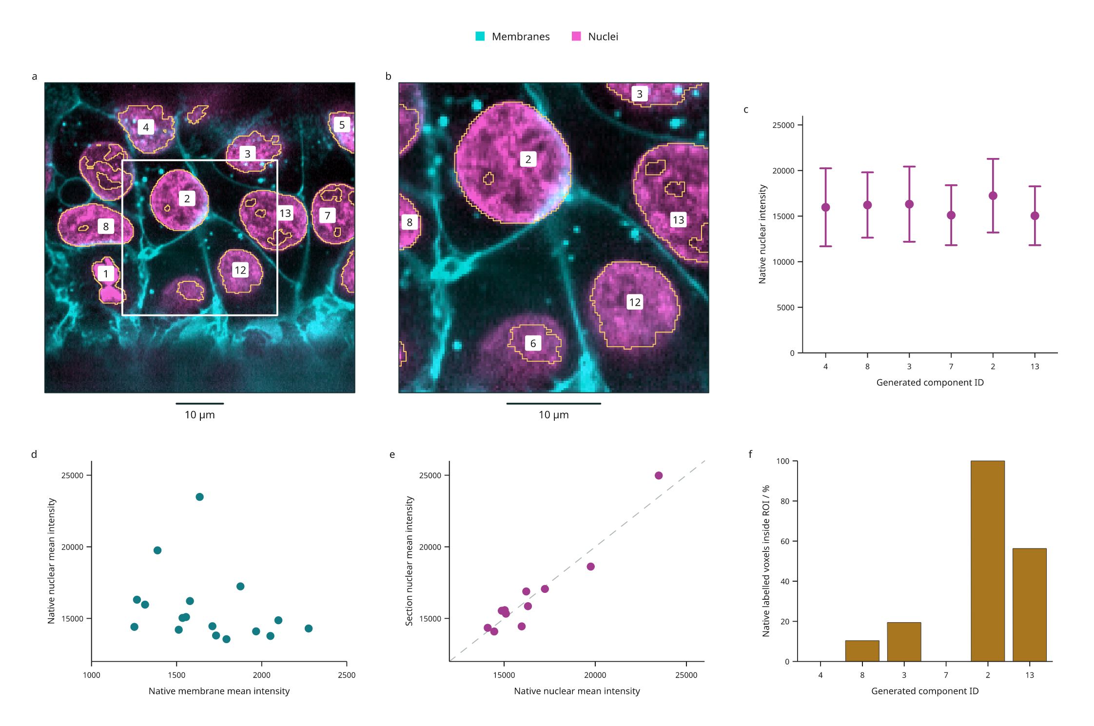
- a: The original two-channel data on a plane tilted 10° from XY. Gold vector contours follow sampled generated labels; dashed edges indicate source/image coverage limits. White marks the intersection of ROI-1 with the plane.
- b: A central 128 × 128 zoom, retaining the overview's 260 nm sampling. Enlargement does not increase resolution. Numeric badges retain original IDs.
- c: Native nuclear mean intensity with population SD of voxel values for the six largest native components that intersect the section. These whiskers describe within-component spread, not standard errors or confidence intervals.
- d: Native mean membrane versus nuclear intensity, one point for each of the 17 generated components. Both values use the same labelled voxels. Colors in the microscopy display and its intensity windows do not affect these means.
- e: Nuclear mean intensity on the section versus the native volume for the same 11 visible IDs. The dashed diagonal indicates equal means. Section means use trilinear intensity interpolation and nearest-neighbour label sampling; native means use original voxels. They describe different spatial samples.
- f: The percentage of native labelled voxels inside ROI-1, in the same six-ID order as c. ROI-1 spans the available Z depth. Native voxel centres are selected using a half-open physical box; this is not a rectangular crop of the oblique image. A zero means that component has no native centres in the ROI.
| Generated ID | Native nuclear mean | Within-component SD | Native labelled voxels inside ROI-1 |
|---|---|---|---|
| 4 | 15964.97 | 4278.56 | 0.00% |
| 8 | 16215.53 | 3582.76 | 10.38% |
| 3 | 16309.13 | 4120.03 | 19.42% |
| 7 | 15099.31 | 3288.26 | 0.00% |
| 2 | 17239.47 | 4039.58 | 100.00% |
| 13 | 15036.94 | 3225.15 | 56.32% |
Values above are rounded for reading; the CSV and JSON retain float64 results. The measurement API guide defines counts, coverage, physical integrals and empty rows.
Processing and interpretation
The recipe generates illustrative labels from the nuclear channel using a 0.5 µm Gaussian, intensity >12,000, 6-connected components and a 20 µm³ minimum volume. Original scan-order IDs persist after filtering. These are not validated nuclei: touching structures can merge, threshold holes persist and dim structures can be missed. Native boundary flags and sampled contour coverage edges are retained in the evidence; a component touching the source boundary may be truncated. Region selection does not establish that an object is complete.
All measurements describe this one image and this processing recipe. Component counts are not independent biological replicates. No background correction, fluorescence intensity calibration, segmentation accuracy, statistical inference or colocalization result is implied by the plots. Means from different channel assays are not calibrated molecular abundance comparisons.
Source and reuse
The source data are CC0, documented in the
pinned scikit-image data notice.
The scikit-image microscopy tutorial
provides calibration and the fourfold XY downsampling history. The TIFF's ImageJ
header does not supply physical spacing, so the importer receives the documented
values explicitly. Zero origin is a chosen local frame, not a microscope stage
position. Source bytes and metadata are locked in
examples/biology/cells3d.lock.json; raw TIFF data are not bundled in the repo.
The derived figure, processing recipe and documentation are MIT, Mark Marosi.