Lines and points¶

Use a line when point order matters, a step for discrete changes, and scatter when the observations should stand independently. Inklet connects line points in supplied order; sort your data explicitly when necessary.

All values below are illustrative. Each snippet can be run independently with core Inklet; PNG preview generation additionally uses the render extra. Run a block from the repository root with .venv/bin/python; each block writes an SVG and PDF. Keep x values sorted for a time or numeric trajectory. A line connects observations in the order supplied and does not fit a model.

Lines¶

A continuous response connects the supplied observations in order.

import math
import inklet as i

time = [n / 4 for n in range(49)]
p = i.plot_spec(x=(0, 12), y=(0, 1.15), height=45)
p.grid(x=False, count=4, stroke='#e1e7e4', stroke_width=.15)
for name, rate, colour in [('Control', .24, '#24698c'),
                           ('Treated', .48, '#288675')]:
    response = [(t, 1 - math.exp(-rate * t)) for t in time]
    p.line(response, name=name, stroke=colour, stroke_width=.45)
p.axes(x='Time / s', y='Normalized response')
p.legend(side='bottom')
doc = i.document(width=110)
doc.add('line', p)
doc.save('line.svg', 'line.pdf')

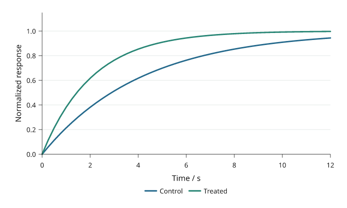
Illustrative first-order responses sampled every 0.25 s. Control and Treated use the same axes and distinct, named colours.

Steps¶

A step holds a value until the next observation. where="post" holds forward, "pre" changes at the preceding x, and "mid" changes halfway between samples. These are supplied values, not a fitted model. Use a step only when the value is held or changes at known transitions; use a line when interpolation between observations is meaningful.

import inklet as i

commands = [(0, 10), (2, 10), (4, 40), (6, 40), (8, 70),
            (10, 70), (12, 30), (14, 30), (16, 55)]
value, response = 10, []
for n in range(65):
    t = n / 4
    target = commands[min(int(t // 2), 8)][1]
    value += .22 * (target - value)
    response.append((t, value))
p = i.plot_spec(x=(0, 16), y=(0, 85), height=45)
p.grid(x=False, count=4, stroke='#e1e7e4', stroke_width=.15)
p.step(commands, where='post', name='Command',
       stroke='#b86443', stroke_width=.45)
p.line(response, name='Simulated response', stroke='#24698c', stroke_width=.45)
p.axes(x='Time / s', y='Output / %').legend(side='bottom')
doc = i.document(width=115)
doc.add('step', p)
doc.save('step.svg', 'step.pdf')

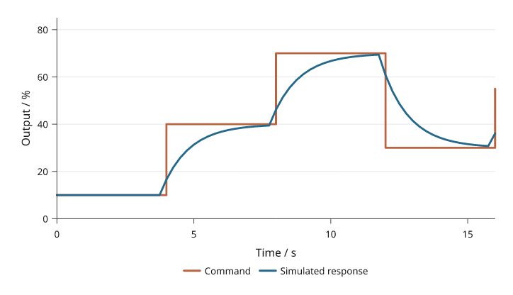
The rust command stays fixed between transitions. The blue simulated response updates every 0.25 s and approaches each new command.

Scatter¶

Scatter shows individual observations without connecting them. size is marker diameter in millimetres, not marker area or a data-coordinate radius. A sequence supplies one size or colour per point; choose the mapping explicitly when encoding another measurement. Avoid encoding a second variable with both size and colour unless a legend makes the mappings unambiguous; overlapping points can hide observations.

import random
import inklet as i

rng = random.Random(28)
points = [(x := rng.uniform(1, 9), 1.2 + .7 * x + rng.gauss(0, .65))
          for _ in range(60)]
p = i.plot_spec(x=(0, 10), y=(0, 9), height=45)
p.grid(x=False, count=4, stroke='#e1e7e4', stroke_width=.15)
p.scatter(points, size=1.3, color='#24698c', name='Samples', fill_opacity=.65)
reference = i.marker('diamond', 2.6).styled(fill='#b86443', stroke='none')
p.marks(reference, [(2, 2.6), (5, 4.7), (8, 6.8)], name='Reference')
p.axes(x='Input / V', y='Response / mV').legend(side='bottom')
doc = i.document(width=110)
doc.add('scatter', p)
doc.save('scatter.svg', 'scatter.pdf')

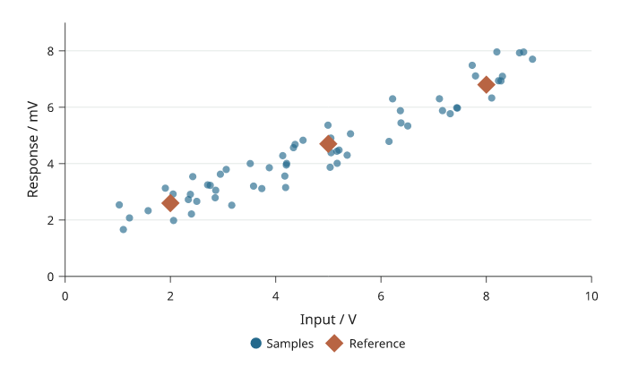
Sixty simulated samples and three explicit reference points. Shape and colour distinguish the references without changing marker size to imply another variable.

Custom markers¶

A reusable drawing can mark each observation. marks() positions the same glyph at data coordinates; its dimensions remain physical. Use the standard scatter(marker=...) options for ordinary symbols.

import math
import inklet as i

points = [(x, 5 * (1 - math.exp(-x / 3))) for x in range(1, 11)]
p = i.plot_spec(x=(0, 11), y=(0, 5.5), height=45)
p.grid(x=False, count=4, stroke='#e1e7e4', stroke_width=.15)
p.line(points, stroke='#b9ceca', stroke_width=.3)
glyph = i.marker('diamond', 2.3).styled(fill='#288675', stroke='none')
p.marks(glyph, points, name='Calibration samples')
p.axes(x='Input / V', y='Output / V').legend(side='bottom')
doc = i.document(width=110)
doc.add('markers', p)
doc.save('markers.svg', 'markers.pdf')

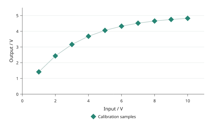
Ten illustrative calibration values use the same diamond glyph. The connecting line follows the supplied values; no model is fitted.

Dumbbells¶

A dumbbell compares two or more values per category. Each series is a dot on the category line, and a grey connector runs from the smallest to the largest value. values has one list per series, in the same shape as grouped bars. None marks a missing value; a category with one value has no connector.

import inklet as i

genes = ['Gad1', 'Slc17a7', 'Pvalb', 'Sst', 'Vip', 'Olig2']
before = [2.1, 3.4, 1.2, 4.0, 2.6, 0.8]
after = [3.9, 2.0, 1.9, 5.2, 3.4, 0.9]
p = i.plot_spec(x=(0, 6), y=genes, height=44)
p.grid(y=False, count=4, stroke='#e1e7e4', stroke_width=.15)
p.dumbbell(genes, [before, after], orient='h', name=['Before', 'After'],
           color=['#24698c', '#b86443'])
p.axes(x='Expression / log CPM').legend(side='top')
doc = i.document(width=100)
doc.add('dumbbell', p)
doc.save('dumbbell.svg', 'dumbbell.pdf')

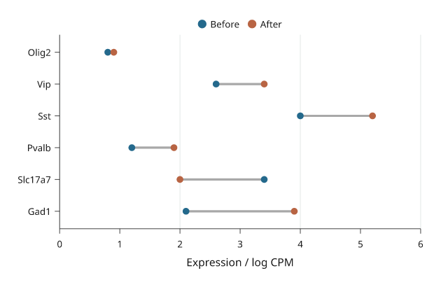
Illustrative expression before and after treatment. The connector length is the change; its direction is read from the dot colours.

Lollipops¶

A lollipop is one value per category: a stem from baseline and a dot at the value. Use it in place of bars when there are many categories.

import inklet as i

pathways = ['Synapse', 'Axon', 'Myelin', 'Immune', 'Vascular', 'Cilia', 'Ribosome']
scores = [2.8, 2.1, 1.4, -0.9, -1.6, 0.6, -2.3]
p = i.plot_spec(x=(-3, 3), y=pathways, height=48)
p.vline(0, stroke='#5f6b7a', stroke_width=.2)
p.lollipop(pathways, scores, orient='h', color='#24698c')
p.axes(x='Enrichment score')
doc = i.document(width=100)
doc.add('lollipop', p)
doc.save('lollipop.svg', 'lollipop.pdf')

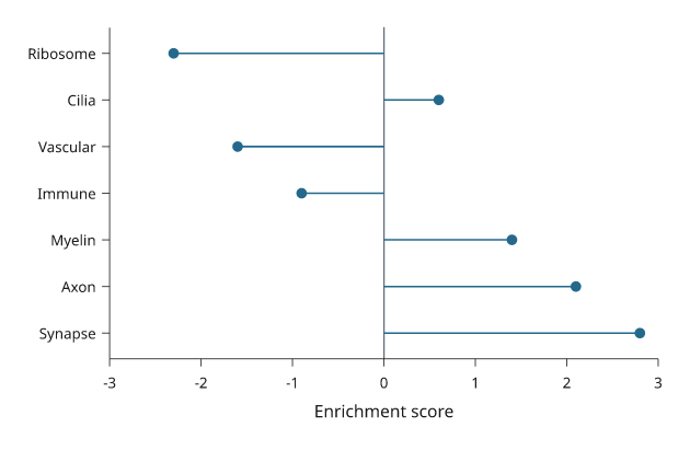
Illustrative enrichment scores. Stems start at the baseline of 0.

Labelled points¶

label_points names many points in one call. Each label is placed at the nearest free position around its point, clear of the marks and of the other labels. A label that has to move further out gets a thin leader line back to its point. Placement happens when the panel is built, so the labels also avoid marks drawn after the call. The placement is deterministic.

import inklet as i
import random

rng = random.Random(7)
genes = [(rng.gauss(0, 1.2), abs(rng.gauss(0, 1.3)) * 1.6) for _ in range(400)]
hits = sorted(genes, key=lambda g: -(g[1] + abs(g[0])))[:8]
names = ['Fos', 'Arc', 'Egr1', 'Npas4', 'Junb', 'Nr4a1', 'Bdnf', 'Homer1']
p = i.plot_spec(x=(-4, 4), y=(0, 8), height=50)
p.scatter(genes, size=.7, color='#c4c9cf')
p.scatter(hits, size=1.0, color='#b86443')
p.label_points(hits, names)
p.axes(x='log2 fold change', y='-log10 p')
doc = i.document(width=90)
doc.add('labelled-points', p)
doc.save('labelled-points.svg', 'labelled-points.pdf')

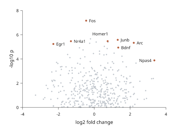
Simulated data. Labels that could not be placed without overlap are listed in the label node's point_labels note under unresolved.

Volcano plots¶

volcano takes log2 fold changes and p-values, one per feature, and draws each feature at (log2 fold change, -log10 p). A point with p below p_threshold (default 0.05) and a fold change of at least fold_threshold (default 1) is "up", one with a fold change of at most -fold_threshold is "down", and every other point is "ns". The "ns" points are drawn first in a pale grey; "up" points are red and "down" points blue. Dashed rules mark the three thresholds; thresholds=False leaves them out.

With labels= (one name per feature), the top significant points with the smallest p-values are named with label_points. Points outside the plot area are not labelled. name= gives legend names for the classes, in the order down, ns, up; None leaves a class out of the legend. A p-value of 0 is drawn at the smallest positive p-value in the data. inklet.plot.volcano_points returns the classes and the ranking without drawing.

import inklet as i
import math
import random

rng = random.Random(11)
fold, pvalues = [], []
for _ in range(1500):
    effect = rng.gauss(0, .5) if rng.random() < .9 else rng.gauss(0, 1.8)
    fold.append(effect)
    pvalues.append(math.erfc(abs(effect * 1.3 + rng.gauss(0, 1)) / math.sqrt(2)))
genes = [f'G{k}' for k in range(1500)]
p = i.plot_spec(x=(-6, 6), y=(0, 16), height=50)
p.volcano(fold, pvalues, labels=genes, top=10, name=('Down', None, 'Up'), size=.8)
p.axes(x='log2 fold change', y='-log10 p').legend(side='right')
doc = i.document(width=90)
doc.add('volcano', p)
doc.save('volcano.svg', 'volcano.pdf')

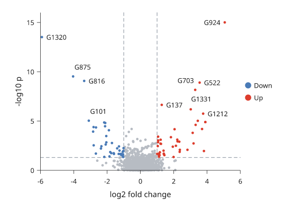
Simulated data. The dashed rules are at a fold change of ±1 and at p = 0.05.

Embedding scatters¶

embedding draws a UMAP or t-SNE style scatter coloured by cluster. It takes (x, y) points and one cluster name per point, and draws them with one scatter call, so from 256 points up they are a single packed marker batch. The points are drawn in a seeded random order, so a cluster listed last does not cover the others; shuffle=False keeps the input order.

Each cluster's name is written at its centre on a paper halo. The centre lies on the data: the member point nearest the cluster's median, which stays on a curved cluster where the mean would not. center='medoid' or 'mean' choose another rule, and inklet.plot.cluster_centers returns the centers without drawing. A name that would overlap a name already placed, or the points of another cluster, moves to the nearest free spot. A name may cover its own cluster. Names that could not clear another cluster's points are listed under covering in the embedding note. arrows='UMAP' draws two short arrows labelled UMAP1 and UMAP2 in the lower-left corner instead of axes. The default colours are Paul Tol's qualitative palettes, and every cluster is recorded for legend().

outline='line' draws a smooth outline round each cluster's core, thin and in the cluster's colour. outline='fill' draws the core as a light tint under the points instead. The core is the region holding the densest outline_core share of the cluster's points (default 0.8). It is found as a threshold on a smoothed density, so it follows a curved cluster, and stray points neither enlarge it nor add islands. A cluster name keeps off other clusters' outlines. It may cross its own outline line, but not the edge of its own tint: a name wider than its core then sits beside the cluster.

import inklet as i
import math
import random

rng = random.Random(5)
centres = {'T cells': (-4.2, 2.6), 'NK': (-1.4, 4.6), 'B cells': (-4.8, -2.6),
           'Monocytes': (2.8, 1.8), 'DC': (4.9, 4.6), 'pDC': (5.8, -.4),
           'Erythroid': (.2, -4.4), 'Platelets': (4.6, -4.4)}
points, clusters = [], []
for name, (cx, cy) in centres.items():
    for _ in range(rng.randint(900, 3200)):
        turn = rng.uniform(0, 2 * math.pi)
        points.append((cx + .55 * math.cos(turn) + rng.gauss(0, .6),
                       cy + .35 * math.sin(turn) + rng.gauss(0, .45)))
        clusters.append(name)
p = i.plot_spec(x=(-8, 8.5), y=(-7, 7), width=60, height=56)
p.embedding(points, clusters, arrows='UMAP', size=.2, outline='line')
doc = i.document(width=76)
doc.add('embedding', p)
doc.save('embedding.svg', 'embedding.pdf')

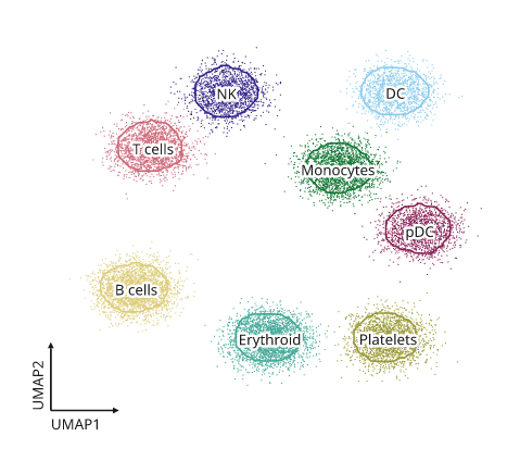
Simulated data. The points are one marker batch; raster=True embeds them as an image instead.

Slope charts¶

A slope chart joins each series' value at two (or a few) positions with a line, and names the series at the ends with its value. highlight= keeps the named series in colour and greys the rest. End labels are spread apart so that they never overlap.

import inklet as i

shares = {'Denmark': [42, 61], 'Spain': [30, 28], 'Italy': [33, 35],
          'France': [45, 52], 'Poland': [25, 41]}
p = i.plot_spec(x=['2015', '2025'], y=(20, 70), height=45, width=26)
p.slope(shares, format='{:.0f}%', highlight=['Denmark', 'Poland'])
p.axis('top', spine=False, tick_size=0)
doc = i.document(width=70)
doc.add('slope', p)
doc.save('slope.svg', 'slope.pdf')

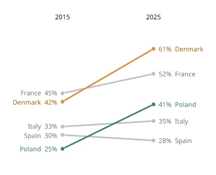
Illustrative shares. The labels are placed outside the plot area.

Bump charts¶

A bump chart follows each series' rank over time. bump ranks the values at each position (largest first) and joins the ranks with smooth S-curves; give ranked=True if the values already are ranks. Use a y scale that runs from the lowest rank at the bottom to rank 1 at the top. numbers=True writes the rank in each dot.

import inklet as i

points = {'Lyon': [3, 5, 8, 9], 'Nice': [8, 6, 5, 3], 'Lens': [5, 9, 7, 8],
          'Metz': [9, 3, 2, 1], 'Brest': [1, 2, 4, 6]}
p = i.plot_spec(x=['2021', '2022', '2023', '2024'], y=(5.5, .5), height=34, width=50)
p.bump(points, numbers=True)
p.axis('top', spine=False, tick_size=0)
doc = i.document(width=80)
doc.add('bump', p)
doc.save('bump.svg', 'bump.pdf')

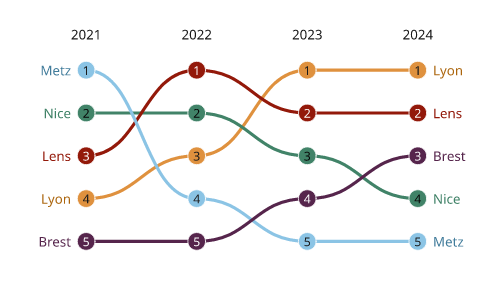
Illustrative scores. inklet.plot.ranks returns the rank table.

Stem plots¶

A stem plot draws a stem from a baseline to a dot at each sample, for a sampled signal on a continuous scale. For one value per category, use lollipop.

import inklet as i
import math

response = [(n, math.exp(-n / 8) * math.cos(n / 2)) for n in range(32)]
p = i.plot_spec(x=(-1, 32), y=(-.8, 1.1), height=34)
p.stem(response)
p.axes(x='Sample n', y='h[n]')
doc = i.document(width=80)
doc.add('stem', p)
doc.save('stem.svg', 'stem.pdf')

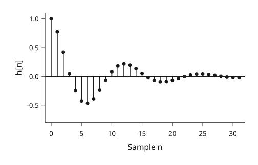
A damped cosine. rule=False leaves out the baseline across the panel.

Parallel coordinates¶

Parallel coordinates give each variable its own vertical axis and draw each record as a line across them. Each axis is scaled to its variable's range. groups= colours the records by group.

import inklet as i
import random

rng = random.Random(3)
records, species = [], []
for s, (length, scale) in enumerate([(5, 1.0), (6.5, 1.4), (8, 1.9)]):
    for _ in range(12):
        l = length + rng.gauss(0, .5)
        records.append([l, l * .45 + rng.gauss(0, .3), 2 + s + rng.gauss(0, .4),
                        scale * l * 10 + rng.gauss(0, 8)])
        species.append(['setosa', 'versicolor', 'virginica'][s])
p = i.plot_spec(x=['Length', 'Width', 'Depth', 'Mass'], height=38, width=62)
p.parallel(records, groups=species)
p.legend(side='right')
doc = i.document(width=90)
doc.add('parallel', p)
doc.save('parallel.svg', 'parallel.pdf')

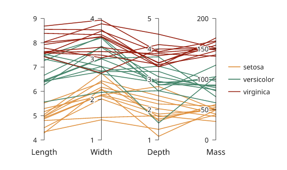
Simulated measurements. A missing value breaks the record's line.

Next steps¶

Compare plot types, configure axes and scales, or arrange several panels. For exact options, see the API.