Linked region maps¶

Experimental: the API may change.

The development preview now joins GeoJSON regions to the same keyed table used by linked bars and scatter plots. Select a region in either map to select its row across all panels, filter regions, save the view, and reconstruct it in Python. This remains an opt-in experimental feature.

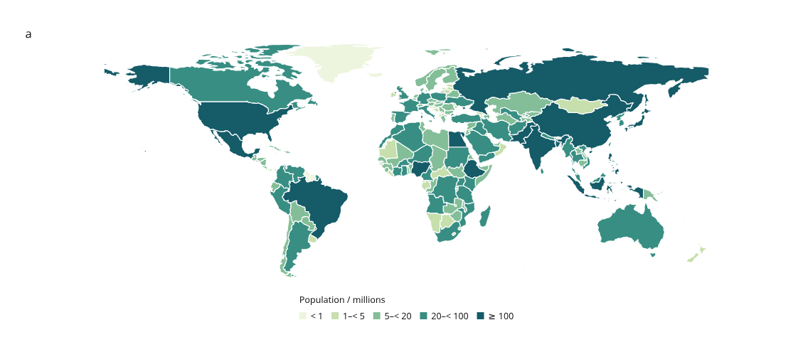
Open the real world and Europe maps · Source data, provenance and recipe

The main example uses real public-domain Natural Earth boundaries and its historical population estimates, mostly dated 2019. Country selection links the world and Europe views. Search by country name or continent; the source year is retained for every row. See the real-map guide for details.

For points, multi-part routes and mixed maps, see GeoJSON features.

Small regression example¶

The four-region figure below is a deliberately simple test fixture. It remains useful for checking expected totals, joins and selection behavior.

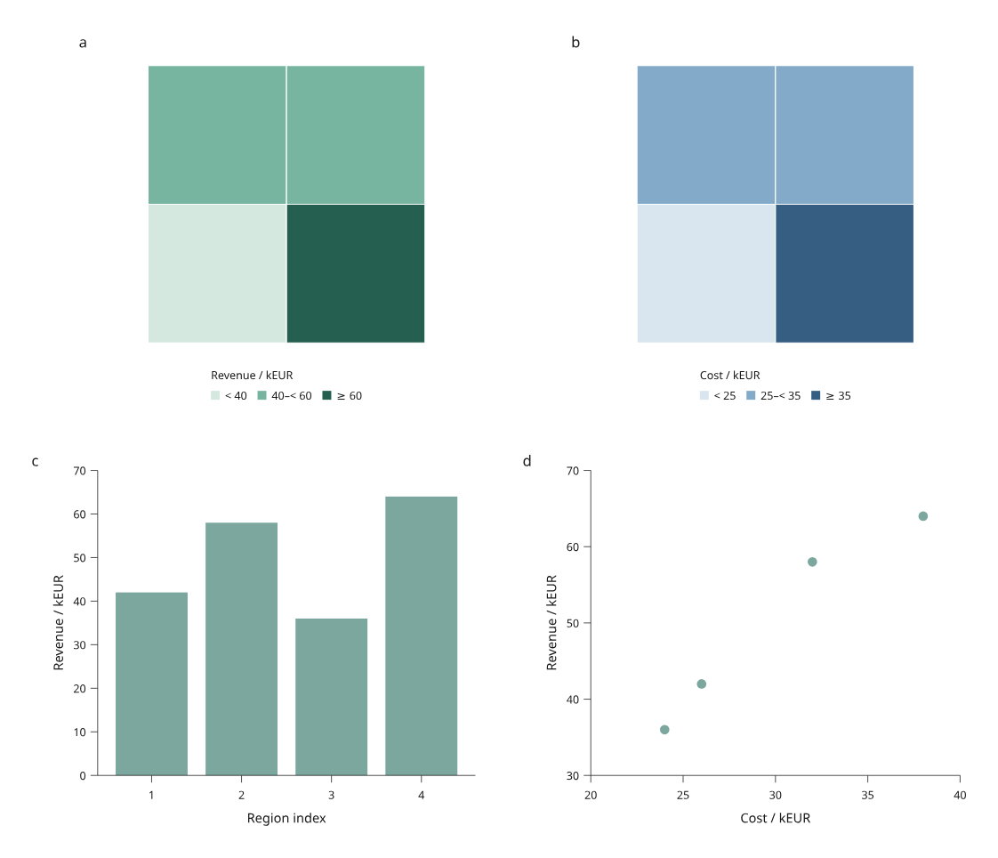
Open the regional analysis · Python example · Original CSV · Original GeoJSON

These four regions are invented rectangles, not administrative boundaries. North is up and east is right. Bar indices 1–4 correspond to Northwest, Northeast, Southwest and Southeast. Total illustrative revenue is 200 kEUR and cost is 120 kEUR. Each North/South group has revenue of 100 kEUR.

A complete linked view¶

1. Click Southeast in either map. Its revenue bar and cost/revenue point share the selection. Hover shows its row ID and the map's joined value.
2. Enter north or south in the ID filter. Hidden selections remain saved and counted; map color bins and legends stay fixed.
3. Pan or zoom the page, then choose Save view. Open saved view restores visibility, selection and viewport.
4. Download vector SVG, or reconstruct the saved view in Python:

python examples/v4/regional_analysis.py --output out/v4-regions
python examples/v4/regional_analysis.py --state /path/to/view.json --output out/v4-restored
# Start with one group visible:
python examples/v4/regional_analysis.py --group North --output out/v4-north

Restored HTML applies the saved state on opening. SVG, Canvas 2D and hybrid backends share the same polygon geometry, clipping, color bins and row identities. Their vector export preserves polygon holes and selection outlines.

Input and projection contract¶

GeoRegions.read(path) reads UTF-8 GeoJSON; GeoRegions.from_geojson(mapping) accepts an already parsed object. Input must be a nonempty FeatureCollection of Polygon or MultiPolygon features with unique, nonempty string feature IDs. Feature IDs must exactly match the table's row IDs. Missing or unmatched geometry fails with the corresponding IDs; no positional join or silent drop occurs. The table supplies values and labels; GeoJSON properties are not used for joins.

The supported coordinate subset follows GeoJSON's longitude/latitude order in decimal degrees. The first polygon ring is the exterior and subsequent rings are holes. See RFC 7946 for the format. This preview accepts two-coordinate positions only, finite longitude in −180…180 and latitude in −90…90, explicit ring closure, at least three distinct vertices and nonzero signed ring area. Either ring orientation is accepted.

Altitude coordinates, null/other geometry types, legacy CRS fields and edges crossing the antimeridian are rejected. Cut crossing polygons before import. Validation checks structure and coordinate bounds; it does not validate or repair self-intersections, hole containment or overlaps between multipolygon parts. Supply valid simple rings, contained holes and nonoverlapping parts. Distinct features may overlap; their picking order is described below.

RegionView uses a fixed flat longitude/latitude view (Plate Carrée) with one physical scale for both degree axes. The map fits inside its measured panel without stretching to the panel's aspect ratio. extent=(west, south, east, north) controls the visible bounds; regions are clipped to that extent. The frame reserves the map area even when it has no axes. Legends are measured and outlined in Python, outside the map area.

This is a geographic display, not an equal-area projection, geodesic measurement or map service. There are no tiles, remote fonts, external network requests or optional GIS dependencies. Other projections and antimeridian/polar handling remain future work. Page zoom changes the viewport, not the geographic extent.

Author a map and scatter panel¶

from pathlib import Path
from inklet.experimental.browser import BrowserFigure, GeoRegions, RegionView, ScatterView
from inklet.selection import KeyedTable

# Use IDs present in your GeoJSON file.
table = KeyedTable("regions", {
    "id": ["west", "east"],
    "revenue": [42, 64],
    "cost": [26, 38],
})
regions = GeoRegions.read("regions.geojson")
figure = BrowserFigure(table, [
    RegionView("map", regions, (0, 0, 2, 1), value="revenue",
               breaks=(40, 60), colors=("#d4e8df", "#78b5a1", "#245f50"),
               value_label="Revenue / kEUR"),
    ScatterView("comparison", "cost", "revenue", (20, 40), (30, 70),
                x_label="Cost / kEUR", y_label="Revenue / kEUR"),
], width=190)
Path("regions.html").write_text(figure.to_html(), encoding="utf-8")
Path("regions.svg").write_text(figure.to_svg(), encoding="utf-8")

Breaks are strictly increasing. Values below the first break use the first color; values equal to a break enter the next bin. A missing/null value keeps its polygon with missing_color and adds a Missing legend entry. A view without value uses one fixed color and no value legend. Filtering changes visibility, never the color scale or legend.

Geometry is copied into immutable tuples. Scene state includes a digest of the source geometry, so changing a hole or boundary invalidates an old scene view even if the table stays the same. Custom table key column names work too.

To export the same row selection at another physical width, explicitly construct that figure and call new_figure.state(selection) using the existing SelectionState. Its viewport starts fitted to the new page. Loading the old page's full browser state into a different scene remains an error.

Holes, islands and boundary picking¶

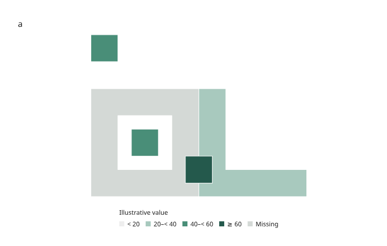
Open the geometry review · Recipe · Original geometry fixture

The gray reserve has a hole. A separate island occupies part of that hole, and another island above the reserve shares its ID. The region to the right is concave. A fourth feature overlaps the reserve and eastern region. All shapes are original simulated test geometry.

Polygons use even-odd filling within each polygon. Their holes remain empty; multipolygon parts share one row ID and highlight together. Picking uses the filled area and includes its boundaries, with a 1e-10 mm numerical boundary tolerance. Shared boundaries and overlapping features choose the later row in the table's source order. Filtering that row exposes the underlying region. Projected physical vertices are rounded to 1e-6 mm; boundary tests use those exported coordinates. Polygon picking deliberately ignores pointer proximity tolerance: a point in a hole or outside a region should not acquire a nearby region. Selection outlines do not enlarge hit areas. All queries remain inside the map clip.

Verification and next work¶

The region regression compares 16,200 indexed queries with the browser's native even-odd point-in-path test, across three backends, visible/filtered/empty states, two page widths and device pixel ratios 1/2. Analytical cases check holes, concavity, shared boundaries, overlap, clipped geometry and multipolygon identity. Browser and Python vector marks match in the tested states; independent 150 dpi rendering of the saved zoomed geometry review matches pixel for pixel.

The regional example also passes direct browser selection, page navigation and saved HTML reopening. This does not complete the regional 4.0 acceptance project: time series, distribution/facet views, explicit table replacement and richer format/projection adapters still need implementation. The previous scatter benchmark does not measure map performance.