Matrices and heatmaps¶

A matrix assigns a colour to each cell. Share the mapping with its colour key, and state the units. A calibrated image or contour field has additional coordinate semantics; see the scientific report and contour guide for the experimental linked workflows.

All values below are illustrative. Each Python block is a complete example using core Inklet. PNG previews additionally use the render extra; PDF export of raster matrices needs Pillow (images or render).

Heatmaps¶

A colour key describes the same mapping as the matrix. colorbar() reuses the matrix ramp and scale. Pass explicit row coordinates to associate each row with its y category. The first category is at the bottom; the next section shows a top-first display. Missing cells use an explicit colour. colorbar(label=) names the bar along its length, turned to read upward beside a vertical bar, which is how journals set a colour bar's name; colorbar(title=) sets the name horizontally above the bar instead.

import inklet as i
p = i.plot_spec(x=['A', 'B', 'C', 'D'], y=['Run 1', 'Run 2', 'Run 3'], height=45)
p.matrix([[2, 5, 7, 3], [4, None, 8, 5], [1, 3, 6, 9]],
         x=['A', 'B', 'C', 'D'], y=['Run 1', 'Run 2', 'Run 3'],
         ramp=i.ramp('tol-ylorbr'), scale=i.linear((0, 10)),
         missing='#e8e8e8', raster=False)
p.axes(x='Condition', y='Run')
p.colorbar(label='Value / a.u.')
doc = i.document(width=105)
doc.add('matrix', p)
doc.save('matrix.svg', 'matrix.pdf')

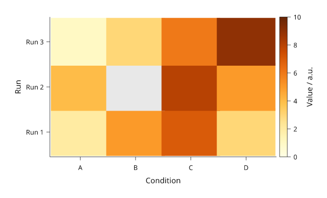
Rendered from the code above. Grey means missing, not zero.

Keep rows rectangular and supply missing= when any value is None or NaN. The colourbar describes the numeric ramp; explain the missing-value colour in the caption. Use the same ramp and scale for comparable panels instead of normalizing each matrix independently.

On a panel with a matrix, an axis with no ticks (ticks=[]) or hidden ticks (labels=False with tick_size=0) draws no spine, since the cells' edge is already the boundary. The axis name is still drawn. Pass spine=True to keep the line.

Row order and comparisons¶

With explicit y= coordinates on matrix(), rows follow those coordinates through the panel's y scale. To put the first named row at the top, reverse the category order on the plot scale and keep the matrix's row coordinates paired with their values. If you reorder the values themselves, reorder their coordinates too.

Without y= on matrix(), row zero starts at the top of the plot area and rows divide the height evenly, independently of the y scale. This differs from the bottom-first categorical axis. Explicit coordinates avoid a silently mislabelled heatmap.

import inklet as i

conditions = ['A', 'B', 'C']
runs = ['Run 1', 'Run 2', 'Run 3']
values = [[1, 2, 3], [4, 5, 6], [7, 8, 9]]
shades, colour_scale = i.ramp('tol-ylorbr'), i.linear((0, 10))
doc = i.document(width=180, columns=2, gap=12,
                 share_plot_margins=True).letters()
for column, labels in enumerate((runs, runs[::-1])):
    p = i.plot_spec(x=conditions, y=labels, height=42)
    p.matrix(values, x=conditions, y=runs,
             ramp=shades, scale=colour_scale, raster=False)
    p.axes(x='Condition')
    p.colorbar(label='Value / a.u.')
    doc.add(f'order-{column}', p, row=0, column=column)
doc.save('matrix-order.svg', 'matrix-order.pdf')

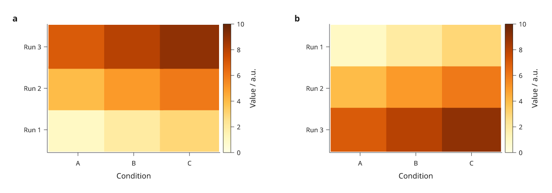
a, First y category at the bottom. b, The category scale is reversed; the input rows and their coordinates stay together. Each named run keeps its values, and both colourbars use the same 0–10 scale.

Numeric sample positions¶

Without x= and y= on matrix(), cells divide the plot area evenly. For measurements at uneven numeric positions, pass sample centres explicitly. Inklet maps those positions through the panel scales and places cell boundaries halfway between neighbouring displayed samples. The outer cells extend by half the adjacent gap. A category scale would give every sample an equal-width slot.

import inklet as i

xs, ys = [0, 1, 4], [0.5, 1.5]
p = i.plot_spec(x=(-0.5, 5.5), y=(0, 2), height=42)
p.matrix([[2, 5, 8], [4, 7, 3]], x=xs, y=ys,
         ramp=i.ramp('tol-ylorbr'), scale=i.linear((0, 10)),
         vector='seamless')
p.scatter([(x, y) for y in ys for x in xs], color='#222222', size=1)
p.axes(x='Sample position / mm', y='Height / mm',
       x_options={'ticks': xs}, y_options={'ticks': ys, 'format': '{:.1f}'})
p.colorbar(label='Value / a.u.')
doc = i.document(width=115)
doc.add('samples', p)
doc.save('matrix-samples.svg', 'matrix-samples.pdf')

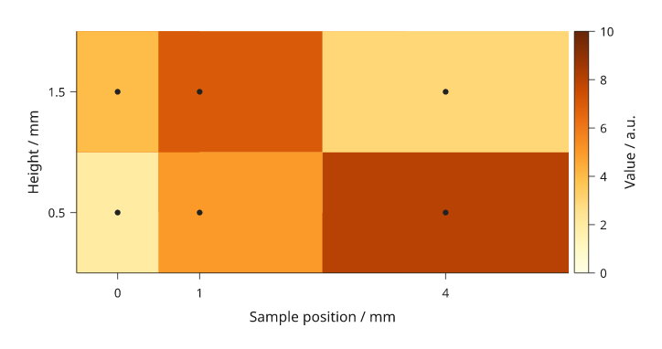
Dots mark supplied sample centres; the colour between samples represents the midpoint-based cell assignment. It does not represent extra observations.

Numeric domains must include the intended cell edges. A singleton row or column fills that panel dimension unless you provide a two-edge interval for it. Uniform edge arrays with one more entry than the number of cells are also accepted. For uneven sampling, supply centres and review the resulting cell boundaries at the final scale.

Default colour ramps¶

Omit ramp= to use the built-in ramps. matrix() chooses one from the data:

• Values on one side of zero use a sequential ramp: matplotlib's magma, reversed, so low values are pale yellow and high values are deep purple. Lightness falls at a steady perceived rate, so equal value steps look equal. The near-black end is omitted so the darkest cells stay distinct from black text and outlines.
• Values on both sides of zero use Paul Tol's blue-white-red diverging ramp (tol-burd), with white at zero.
• center= selects the diverging ramp and puts white at that value.

Without scale=, the colour scale spans the data. For a diverging ramp it is made symmetric about the centre, so equal distances above and below the centre get equally strong colours. colorbar() reads the same scale. An explicit scale= is used as given; if its domain includes zero, the diverging ramp is chosen. center= and scale= cannot be combined.

import inklet as i

levels = [[0.4, 1.1, 2.3, 3.0], [0.9, 2.2, 3.6, 4.1], [1.5, 2.8, 4.4, 5.2]]
change = [[-1.8, -0.6, 0.2, 1.4], [-0.9, 0.1, 0.8, 2.1], [-0.2, 0.7, 1.6, 2.6]]
conditions = ['A', 'B', 'C', 'D']
runs = ['Run 1', 'Run 2', 'Run 3']
doc = i.document(width=150, columns=2)
panels = [('level', levels, 'Level / a.u.'), ('change', change, 'Change / a.u.')]
for column, (name, values, key) in enumerate(panels):
    p = i.plot_spec(x=conditions, y=runs, height=30)
    p.matrix(values, x=conditions, y=runs, raster=False)
    p.axes(x='Condition', y='Run')
    p.colorbar(label=key)
    doc.add(name, p, row=0, column=column)
doc.save('matrix-default-ramps.svg', 'matrix-default-ramps.pdf')

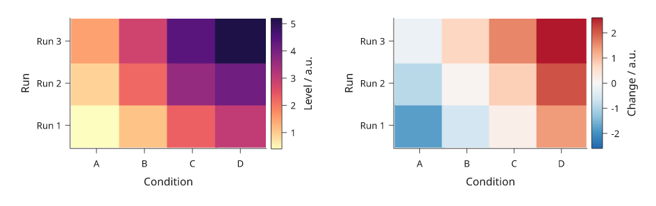
Left: sequential default. Right: diverging default with white at zero.

An explicit ramp= keeps its previous meaning. Without scale=, the values are read as fractions of the ramp from 0 to 1. Pass ramp=i.ramp('magma') or ramp=i.ramp('tol-burd') to use either palette with your own scale.

Choose vector or raster cells¶

These options change the representation of the matrix layer. Axes, labels and colourbars remain vector artwork.

Ordinary vector cells overlap slightly to hide antialiasing seams; set overlap=0 for exact abutting rectangles. Batched and seamless modes default to zero overlap and reject a nonzero override. Raster colour mapping uses 256 ramp levels; batched vector colours are not quantized.

Nearest-cell rendering is the default. Explicit raster=True, interpolation='linear', samples=4 interpolates scalar values before applying the colour ramp. samples must be an integer from 2 to 16; linear interpolation requires uniform displayed spacing and the default vector='cells'. Missing values affect the interpolation footprint instead of being filled with zero. Use interpolation only when the figure should show a continuous field, and describe that choice in the caption.

Dendrograms¶

dendrogram draws the merge tree of a hierarchical clustering as elbows. It takes a SciPy linkage matrix, one row [a, b, distance, count] per merge, or a nested sequence of leaf names such as (('a', 'b'), ('c', 'd')). A nested tree has no distances, so each merge is drawn one unit above its tallest child. labels= names the leaves of a linkage in their original order.

With orient='v' (default) the leaves run along x and the merge heights on y. With orient='h' the leaves run along y and the heights on x. Reverse the height domain to grow the tree the other way: x=(height, 0) puts the root on the left and the leaves on the right, next to a heatmap.

To line the tree up with a heatmap, use the same band scale for both. The band's categories must be in the dendrogram's leaf order, and dendrogram raises an error when they are not. inklet.plot.dendrogram_layout(tree, labels=...) returns that order in leaves; reorder the matrix rows and columns to match. On a y band the first leaf is at the bottom. row and column align the panels on their plot areas.

threshold= gives each subtree whose merges are all below that height its own colour and draws the merges above it in the ink.

import inklet as i
from inklet.plot import dendrogram_layout

genes = ['Fos', 'Arc', 'Egr1', 'Npas4', 'Junb', 'Gfap', 'Aqp4', 'Mbp', 'Plp1', 'Mog']
samples = ['S1', 'S2', 'S3', 'S4', 'S5', 'S6']
values = [[1.1, .8, -.8, -2, .1, -.7], [1.9, 1.3, -.5, -1.4, .3, 0],
          [1.2, 1.3, -1.4, -1.3, .4, .1], [1.4, 2, -1, -1.4, .3, -.1],
          [1.4, 1.1, -.3, -1.2, .3, .3], [-.3, -.9, 1.2, 2, -.8, -.1],
          [-.8, 0, 1.1, .3, -.1, -.2], [-.1, .4, -.2, .1, 1.4, 1.9],
          [.5, .2, -.5, .3, 1.8, 1], [-.2, .6, -.3, -.1, 1.7, 1.4]]
# Average-linkage Euclidean clustering of the rows and of the columns.
gene_tree = [[7, 9, .66, 2], [1, 4, .68, 2], [2, 3, .87, 2], [8, 10, 1.12, 3],
             [11, 12, 1.13, 4], [0, 14, 1.43, 5], [5, 6, 2.11, 2],
             [13, 15, 3.19, 8], [16, 17, 4.06, 10]]
sample_tree = [[4, 5, 1.57, 2], [0, 1, 1.7, 2], [2, 3, 2.3, 2], [6, 7, 3.82, 4],
               [8, 9, 5.51, 6]]
rows = list(dendrogram_layout(gene_tree, labels=genes).leaves)
cols = list(dendrogram_layout(sample_tree, labels=samples).leaves)
cells = [[values[genes.index(g)][samples.index(s)] for s in cols] for g in rows]

heat = i.panel(36, 50, x=cols, y=rows)
heat.matrix(cells, x=cols, y=rows, ramp=i.ramp('tol-sunset'),
            scale=i.linear((-2, 2)), raster=False)
heat.axis('bottom', spine=False).axis('right', spine=False)
heat.colorbar(label='z-score', side='bottom')
left = i.panel(12, 50, x=(4.06, 0), y=rows)
left.dendrogram(gene_tree, labels=genes, orient='h', threshold=2)
top = i.panel(36, 8, x=cols, y=(0, 5.51))
top.dendrogram(sample_tree, labels=samples)
fig = i.figure(width=90)
fig.add(i.column([top, i.row([left, heat], gap=1)], gap=1, align='right'))
fig.save('dendrogram.svg', 'dendrogram.pdf')

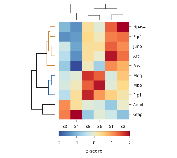
Illustrative values. The gene tree is coloured below a height of 2, which gives two coloured groups. The Gfap and Aqp4 merge, at 2.11, is above the threshold and is drawn in the ink.

Dot plots¶

dotplot draws one circle per cell, with two values per cell. The circle's area shows one value, such as the fraction of cells that express a gene. Its colour shows another, such as the mean expression. Both axes are band scales, and size[r][c] is drawn at the rth y category and the cth x category. Colours use the default matrix ramps, or ramp=, scale= and center= as matrix takes them. A cell whose value is None or NaN draws nothing.

The largest value gets a circle 0.9 of the band step across by default. Set top= for the value drawn at full size and diameter= for its width. Area is proportional to value, so a circle for half of top has half the area. colorbar() explains the colours, and size_key() draws reference circles with their values. inklet.plot.area_scale(top, diameter) gives the same size mapping for a scatter: size the points with it and pass it to size_key(source).

A dendrogram on the same band categories lines up with the rows, as it does with a heatmap.

import inklet as i
import random

genes = ['Cd3e', 'Cd4', 'Cd8a', 'Nkg7', 'Gzmb', 'Ms4a1', 'Cd79a', 'Lyz2', 'Csf1r']
markers = {'CD4 T': {'Cd3e', 'Cd4'}, 'CD8 T': {'Cd3e', 'Cd8a', 'Gzmb'},
           'NK': {'Nkg7', 'Gzmb'}, 'B': {'Ms4a1', 'Cd79a'},
           'Mono': {'Lyz2', 'Csf1r'}, 'DC': {'Lyz2', 'Cd4'}}
tree = ((('CD4 T', 'CD8 T'), 'NK'), ('B', ('Mono', 'DC')))
order = list(i.plot.dendrogram_layout(tree).leaves)
rng = random.Random(3)
fraction = [[rng.uniform(.6, .95) if g in markers[c] else rng.uniform(0, .25)
             for g in genes] for c in order]
mean = [[rng.uniform(1.6, 3) if g in markers[c] else rng.uniform(0, .8)
         for g in genes] for c in order]

dots = i.panel(38, 26, x=genes, y=order)
dots.dotplot(fraction, mean)
dots.axis('bottom', rotate=90, spine=False).axis('right', spine=False)
dots.colorbar(label='Mean expression', length=14)
dots.size_key(title='Fraction', format='{:.0%}')
side = i.panel(9, 26, x=(3, 0), y=order)
side.dendrogram(tree, orient='h')
fig = i.figure(width=90)
fig.add(i.row([side, dots], gap=1))
fig.save('dotplot.svg', 'dotplot.pdf')

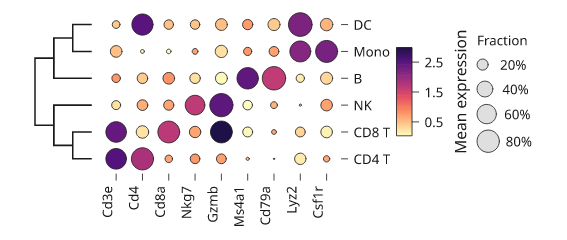
Illustrative values. Each cluster has two or three marker genes with a high fraction and a high mean. The cluster tree is a nested sequence, so its merge heights are levels rather than distances.

Clustered matrices¶

inklet.plot.linkage(rows, method=, metric=) clusters the rows of a table hierarchically without SciPy. It returns the merge table SciPy returns, so dendrogram and dendrogram_layout take it unchanged. The methods are "average" (default), "single", "complete", "weighted" and "ward". The metrics are "euclidean", "correlation", "cosine", "cityblock", a function, or "precomputed" for a distance matrix. cut(link, k) returns one cluster number per row, numbered in the tree's leaf order, so once the matrix is reordered by dendrogram_layout(link).order each cluster is a run of consecutive rows.

clusters(groups) draws a box on the diagonal around each run of equal labels in groups, one label per matrix row from the top. highlight= draws chosen clusters in red over the others, and labels=True names each cluster to the right of the matrix.

To magnify part of the matrix, pass zoom=(x0, x1, y0, y1) to inset. Style keywords colour the window; connector= styles the connector lines alone, for example dashed.

import inklet as i
import random
from inklet.plot import cut, dendrogram_layout, linkage

rng = random.Random(5)
n = 40
community = [k % 5 for k in range(n)]
rng.shuffle(community)
weights = [[0.0] * n for _ in range(n)]
for a in range(n):
    for b in range(a):
        linked = rng.random() < (0.7 if community[a] == community[b] else 0.05)
        weights[a][b] = weights[b][a] = linked * rng.uniform(0.3, 1)
link = linkage(weights, metric='correlation')
order = dendrogram_layout(link).order
groups = [cut(link, 5)[k] for k in order]
adjacency = [[weights[a][b] for b in order] for a in order]
scale = i.linear((0, 1))
m = i.panel(50, 50, x=(0, n), y=(n, 0))
m.matrix(adjacency, scale=scale).clusters(groups, highlight=2, labels=True)
zoom = i.panel(24, 24)
zoom.matrix([row[8:16] for row in adjacency[8:16]], scale=scale)
m.inset(zoom, side='right', width=None, zoom=(8, 16, 8, 16), stroke='#c9352b',
        stroke_width=0.35, connector={'stroke_dash': (1, 0.6)})
m.colorbar(side='bottom', label='weight', length=24)
fig = i.figure(width=100)
fig.add(m.build())
fig.save('clusters.svg', 'clusters.pdf')

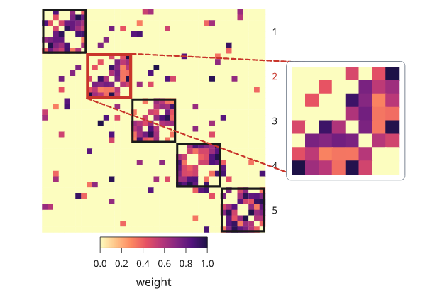
Simulated network of five communities. The rows are in the dendrogram's leaf order, so each community is one box on the diagonal; the inset magnifies the highlighted one.

Clustermaps¶

inklet.clustermap(values) builds the whole clustered heatmap. It clusters the rows and columns, reorders the matrix, and adds both dendrograms, annotation strips, a colorbar and the row and column names when there is room for them. standardize="rows" z-scores each row first. k= cuts the row tree into clusters, colours the tree by cluster, and separates the clusters with rules. When the matrix is square with the same order on both axes, such as a correlation matrix, the clusters are boxed on the diagonal instead. row_color= and col_color= map a track name to one value per row or column: colours, or categories that are coloured from the palette and named in a legend.

import inklet as i
import random

rng = random.Random(7)
genes = ['Fos', 'Arc', 'Egr1', 'Npas4', 'Junb', 'Gfap', 'Aqp4', 'Aldh1l1',
         'Mbp', 'Plp1', 'Mog', 'Olig2']
samples = [f'S{k}' for k in range(1, 10)]
condition = ['ctrl', 'ctrl', 'ctrl', 'KA', 'KA', 'KA', 'LPS', 'LPS', 'LPS']
signal = {'ctrl': 8, 'KA': 0, 'LPS': 4}
expression = [[rng.gauss(2.5 if signal[c] <= g < signal[c] + 4 else 0, 0.8)
               for c in condition] for g in range(12)]
cm = i.clustermap(expression, rows=genes, columns=samples, standardize='rows', k=3,
                  col_color={'condition': condition}, label='z-score', width=36)
fig = i.figure(width=100)
fig.add(cm)
fig.save('clustermap.svg', 'clustermap.pdf')

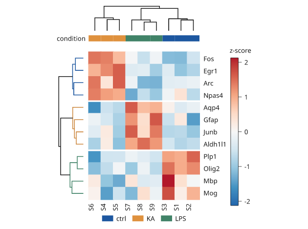
Simulated expression. Three gene modules respond to three conditions, and the row tree is coloured by the three clusters k=3 cuts.

Correlograms¶

correlogram(r, name) draws a correlation matrix as a triangle of glyphs. Each glyph's area is proportional to |r| and its colour is r on a diverging ramp fixed from -1 to 1, so colorbar() shows the full scale. inklet.plot.correlation(table) computes Pearson r between rows, or columns with by="columns". triangle="lower" (default) and "upper" draw each pair once without the diagonal. shape= is "circle", "square" or "tile", and values=True writes r in each glyph.

import inklet as i
import random
from inklet.plot import correlation

rng = random.Random(8)
genes = ['Gad1', 'Gad2', 'Slc32a1', 'Pvalb', 'Sst', 'Vip', 'Slc17a7', 'Satb2']
base = [[rng.gauss(0, 1) for _ in range(40)] for _ in range(3)]
module = [0, 0, 0, 1, 1, 2, 2, 2]
sign = [1, 1, 1, 1, -1, -1, 1, 1]
table = [[sign[g] * base[module[g]][k] + rng.gauss(0, 0.7) for k in range(40)]
         for g in range(8)]
r = correlation(table)
dots = i.panel(40, 40).correlogram(r, genes).colorbar(label='r', length=24)
tiles = i.panel(40, 40).correlogram(r, genes, triangle='upper', shape='tile', values='{:.1f}')
fig = i.figure(width=130)
fig.add(i.row([dots, tiles], gap=14, align='top'))
fig.save('correlogram.svg', 'correlogram.pdf')

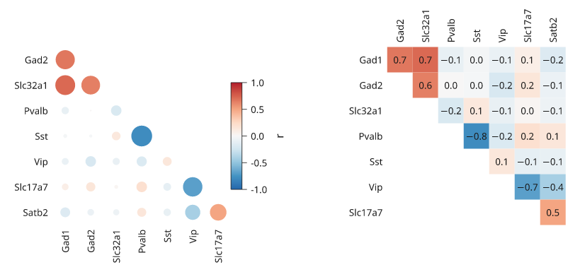
Simulated expression of three gene modules. Colour gives the sign of r and circle area its strength.

Next steps¶

Compare plot types, configure axes and scales, or arrange several panels. For exact options, see the API.