Networks and hierarchies¶

These plots fill a panel's plot area with a structure rather than plotting against its scales: a tree of nested groups, or nodes joined by weighted edges. Sizes are in millimetres like everything else, and every plot here leaves a note on its node with the geometry it drew, so a test can check the picture against the numbers.

Hierarchy input¶

treemap, icicle and sunburst take the same hierarchy, in any of three spellings. inklet.plot.hierarchy(data) reads it and returns the tree, so you can check what a plot will draw.

• A nested mapping: {"cortex": {"L5": {"ET": 40, "IT": 65}, "L6": 80}}. A leaf is a number; a list of names is leaves of 1 each. Several top-level keys share an unnamed root.
• (name, children) tuples: ("cortex", [("L5", [("ET", 40), ("IT", 65)]), ("L6", 80)]).
• A table of (name, parent[, value]) rows, with None as the root's parent.

A group's value is the sum of its children. Nodes are found by name, or by path (a tuple of names from below the root) when names repeat.

Treemaps and sunbursts¶

treemap tiles the plot area with one rectangle per leaf, its area proportional to the value, using the squarified layout so the cells stay close to square. Groups become pale plates with their name in a header strip. sunburst draws the same tree as rings: the root in the middle, each level one ring further out, and each node's angle proportional to its value.

Colours follow the branch: each child of the root gets a colour from the theme's palette, lightened for deeper levels. color= takes a list per branch, a mapping of names to colours, or one colour. highlight= draws the named nodes in red and everything else pale. Labels are written only where they fit inside their cell.

import inklet as i

cortex = {'cortex': {'L2/3 IT': 120, 'L4/5 IT': 90, 'L5 ET': 40, 'L6 IT': 55, 'L6 CT': 70,
          'Inhibitory': {'Pvalb': 45, 'Sst': 38, 'Vip': 22, 'Lamp5': 18, 'Sncg': 6},
          'Non-neuronal': {'Astro': 50, 'Oligo': 64, 'OPC': 15, 'Micro': 12}}}
tree = i.panel(60, 40).treemap(cortex, values='{:.0f}')
rings = i.panel(40, 40).sunburst(cortex)
fig = i.figure(width=120)
fig.add(i.row([tree, rings], gap=6))
fig.save('treemap.svg', 'treemap.pdf')

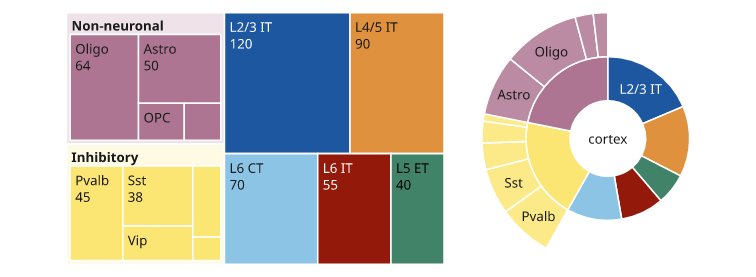
Illustrative counts. The inhibitory and non-neuronal groups are plates with their children inside; the sunburst's inner ring is the same groups.

Clustering levels¶

icicle draws each level of the tree as a row of bars whose widths are the values. With gap= the levels separate and pale fans join each node to its children, which is the usual way to show how clusters split from one level of resolution to the next. orient="h" (default) runs the levels as columns from left to right; "v" runs them as rows from the top.

highlight= marks a lineage in red. labels="highlight" names only the highlighted nodes, or pass the names or paths to label. Long names go outside the bars with a leader tick. levels=True numbers the levels on the left and counts=True writes how many nodes each level has on the right, with the number of highlighted nodes in red.

import inklet as i

levels = {'1': {'1.1': {'1.1.1': 8, '1.1.2': 5}, '1.2': {'1.2.1': 6, '1.2.2': 3, '1.2.3': 2}},
          '2': {'2.1': {'2.1.1': 7, '2.1.2': 7},
                '2.2': {'2.2.1': 4, '2.2.2': 3, '2.2.3': 2, '2.2.4': 2}}}
lineage = [('2',), ('2', '2.2'), ('2', '2.2', '2.2.2')]
p = i.panel(40, 50)
p.icicle(levels, gap=3, highlight=lineage, labels='highlight', levels=True, counts=True)
fig = i.figure(width=70)
fig.add(p.build())
fig.save('icicle.svg', 'icicle.pdf')

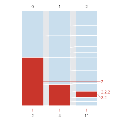
Illustrative clusters. The highlighted lineage is red at every level, and the counts on the right give the number of clusters and highlighted clusters per level.

Weighted networks¶

network draws nodes and weighted edges. nodes is a list of names or a mapping of name to value; edges are (source, target), (source, target, weight) or (source, target, weight, category) rows.

• Layout. layout="circular" (default) puts the nodes on one ring from twelve o'clock, in input order or order=, and bows each edge towards the centre. "force", "layered" and "tree" use the solvers of inklet.graph, stretched to fill the area, with straight edges.
• Nodes. A node's area is proportional to its value, with a floor so small nodes stay visible; size= (a mapping or one value per node) gives the values when nodes is a list. shape="square" draws rounded squares. groups= colours nodes by category, and legend() names the groups. color= is the fill of ungrouped nodes, or a mapping of node or group names to colours.
• Edges. Width is proportional to weight, from a hairline floor up to width (1.6 mm). Lighter edges are drawn first. Edge categories get their own colours and legend entries; edge_color= maps categories to colours. arrows=True adds heads, and two opposite edges bow to opposite sides.

width_key() explains the edge widths with reference lines, and size_key() the node areas. Names are written inside a node when they fit and outside it otherwise, at label_size.

import inklet as i

neurons = {'AVA': 60, 'AVB': 34, 'AVD': 22, 'AVE': 28, 'PVC': 25, 'RIM': 18,
           'AIB': 16, 'DVA': 12, 'RIB': 10, 'SMD': 9}
synapses = [('AVA', 'AVD', 5200, 'chemical'), ('AVD', 'AVA', 1800, 'chemical'),
            ('AVE', 'AVA', 4100, 'chemical'), ('AVB', 'PVC', 900, 'gap junction'),
            ('PVC', 'AVB', 3300, 'chemical'), ('RIM', 'AVA', 2500, 'gap junction'),
            ('AIB', 'RIM', 1600, 'chemical'), ('AIB', 'AVE', 700, 'chemical'),
            ('DVA', 'AVB', 450, 'gap junction'), ('RIB', 'AVE', 300, 'chemical'),
            ('SMD', 'RIB', 1200, 'gap junction'), ('AVA', 'SMD', 200, 'chemical')]
command = {n: 'command' for n in ('AVA', 'AVB', 'AVD', 'AVE', 'PVC')}
p = i.panel(55, 55)
p.network(neurons, synapses, shape='square', diameter=6, arrows=True,
          groups={n: command.get(n, 'other') for n in neurons},
          color={'command': '#c0392b', 'other': '#bdbdbd'},
          edge_color={'chemical': '#4d4d4d', 'gap junction': '#e69f00'})
p.width_key(title='synapses', values=[5000, 2000, 500], format='{:,.0f}')
p.legend(side='bottom')
fig = i.figure(width=89)
fig.add(p.build())
fig.save('network.svg', 'network.pdf')

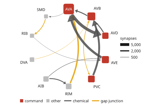
Illustrative weights. Command interneurons are red, and the width key reads edge weight in synapses.

Chord and arc diagrams¶

chord puts groups on a ring as arcs proportional to their totals and joins them with ribbons proportional to the flows. matrix[i][j] is the flow from group i to group j. Undirected (the default), a ribbon is matrix[i][j] wide at i and matrix[j][i] wide at j. directed=True counts each group's outgoing and incoming flows and points each ribbon at its target.

arc_diagram puts the nodes in a row and draws each edge as a half-ellipse above it, with the same node and edge encodings as network. With directed=True, edges that run right to left hang below the row.

import inklet as i

areas = ['V1', 'LM', 'AL', 'RL', 'AM', 'PM']
flows = [[0, 18, 9, 7, 4, 11], [16, 0, 8, 3, 2, 5], [7, 9, 0, 6, 3, 2],
         [5, 2, 7, 0, 6, 3], [3, 1, 2, 7, 0, 8], [12, 4, 1, 2, 9, 0]]
chords = i.panel(45, 45).chord(flows, areas, directed=True)
genes = ['Rbfox3', 'Snap25', 'Syt1', 'Gad1', 'Gad2', 'Slc32a1', 'Olig2', 'Sox10', 'Mbp']
pairs = [('Rbfox3', 'Snap25', 8), ('Snap25', 'Syt1', 9), ('Rbfox3', 'Syt1', 5),
         ('Gad1', 'Gad2', 9), ('Gad2', 'Slc32a1', 7), ('Gad1', 'Slc32a1', 6),
         ('Olig2', 'Sox10', 8), ('Sox10', 'Mbp', 9), ('Olig2', 'Mbp', 4),
         ('Syt1', 'Gad1', 2), ('Snap25', 'Mbp', 1)]
module = {g: 'neuronal' for g in genes[:3]}
module.update({g: 'inhibitory' for g in genes[3:6]}, **{g: 'glial' for g in genes[6:]})
arcs = i.panel(70, 28).arc_diagram(genes, pairs, groups=module)
arcs.width_key(title='co-expression').legend(side='bottom')
fig = i.figure(width=160)
fig.add(i.row([chords, arcs], gap=8))
fig.save('chord.svg', 'chord.pdf')

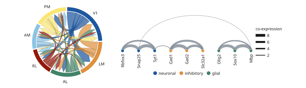
Illustrative flows. In the chord diagram each ribbon is coloured by its source and points at its target.

Next steps¶

Cluster a matrix, compare plot types, or arrange several panels. For exact options, see the API.