

On this page
Shared oblique planes in a real biological volume
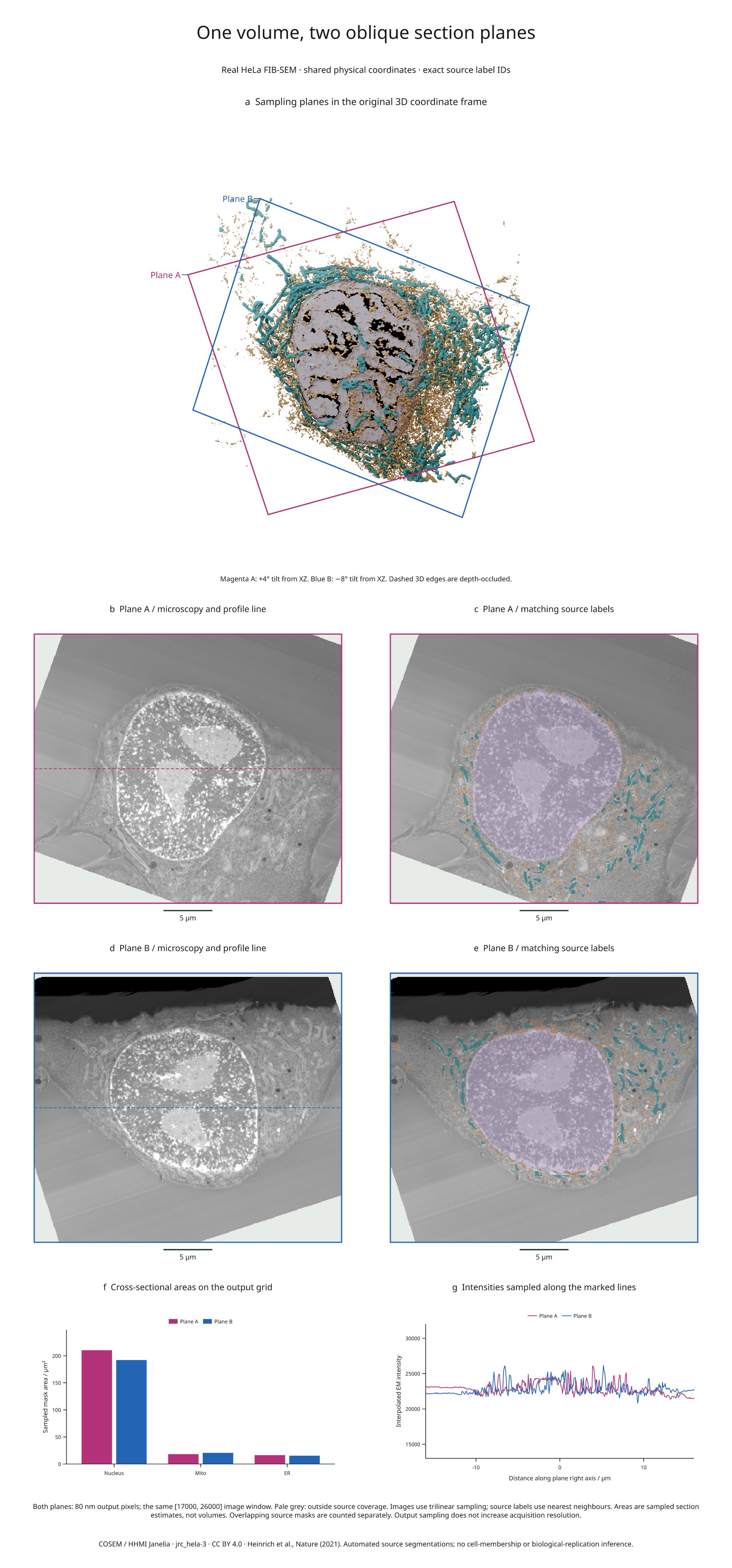
Seven panels connect two physical planes through a COSEM HeLa microscopy crop: their positions in the GPU-rendered organelle scene, raw intensity sections, matching source labels, sampled cross-sectional areas and intensity profiles.
Full-size figure · Executable recipe · Sampling and measurement evidence

Reproduce it
From 4.3 the example imports from inklet.volume; the inklet.experimental
paths still work and, from 4.4, warn.
From the v4.9.0 release checkout with Blender 4.2 or 4.5 LTS:
git clone --branch v4.9.0 https://github.com/Mapika/inklet.git
cd inklet
python -m pip install -e '.[volume,render]'
python -m pip install -r examples/biology/requirements.txt
python examples/oblique_biology.py --blender /path/to/blender
The recipe reuses the real-microscopy example's hash-locked
source cache in out/real-biology/source.n5/. If missing, it downloads the
approximately 56.6 MB of recorded objects. Use --source-cache to choose another
location. A separately cached organelle scene fits the complete sampling planes;
the recipe checks every plane corner against the saved camera frame. The scene,
new figure and sections.json are written to out/oblique-biology/.
What is shared across the panels
Both planes pass through the physical centroid of source nucleus label 1. Plane A has an in-XZ rotation of +20° and a tilt of +4° from XZ; plane B uses −18° and −8°. Their full bases and world corners are recorded, so the recipe does not depend on an implicit Euler-angle convention.
Each output is 351 × 401 pixels, spaced 0.08 × 0.08 µm. The physical
rectangle is 28.08 × 32.08 µm in height/width order. The source level remains
s4, with ZYX spacing 0.05184 × 0.064 × 0.064 µm. No source axis is stretched.
- Panel a projects the exact sampling rectangles through the saved Blender camera. Solid edges are visible; dashed edges are depth-occluded. The organelle geometry remains intact; these are section markers, not cutaways.
- Panels b–e reuse the corresponding plane for raw microscopy and every label
mask. Intensity interpolation is trilinear; integer labels use nearest
neighbours. The image window is
[17000, 26000], and mask color has 55% weight. - Panel f compares foreground mask areas on each output sampling grid. Source masks overlap and are measured separately. These estimates are not volumes.
- Panel g uses output row 175, marked by a dashed line on each raw section. Horizontal position is physical distance along that plane's right direction. Invalid samples break the plotted line rather than becoming zero intensity.
Pale grey areas in the section panels lie outside source coverage. They are not included in area measurements. Label IDs, per-mask sampled areas, validity masks for the profiles and unwindowed profile values are saved in the evidence file. The oblique-section API guide explains these contracts.
| Plane | Valid samples | Nucleus mask area | Mitochondrial mask area | ER mask area |
|---|---|---|---|---|
| A | 131,502 / 140,751 | 210.2144 µm² | 18.2656 µm² | 16.3328 µm² |
| B | 130,876 / 140,751 | 192.0448 µm² | 20.6272 µm² | 15.3088 µm² |
Interpretation and reuse
The data and automated labels are from COSEM / HHMI Janelia, jrc_hela-3. These are visualizations of supplied segmentations, not ground truth or a reanalysis of the publication. The fixed crop does not infer cell membership, complete organelles or independent biological replication. Section areas depend on the chosen plane and output pixel grid; no uncertainty model is supplied.
Data and derived figure: CC BY 4.0. Code: MIT. Attribution, source checksums and known segmentation overlaps are documented in the original example and third-party notices. Publication: Heinrich et al., Whole-cell organelle segmentation in volume electron microscopy, Nature 599, 141–146 (2021). The new processing adds oblique resampling, plane annotations, mask-area estimates and line profiles to the same source crop.