Reusable plots and composition¶

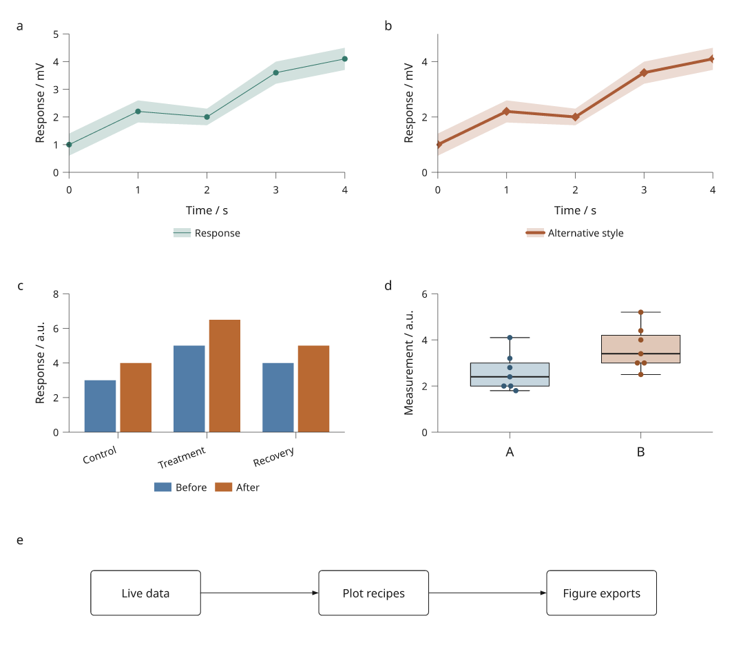
Make a paired comparison without maintaining two copies of the plotting code. This tutorial combines line and point recipes, gives one copy a different visual treatment, then updates both from shared measurements.

Available in the published 4.9.0 release; see the installation guide. Run the Python blocks in order after your first figure. The core installation is sufficient for the SVG/PDF outputs.

Complete Python recipe · Open the native figure viewer · Narrow 150 mm version

All measurements are illustrative. The response bounds are supplied ranges, not inferred confidence intervals. The same diagram and plotting recipes produce both page widths without scaling their text or strokes.

Combine mark recipes¶

import inklet as i

measurements = i.dataset({'x': [0, 1, 2], 'y': [1, 3, 2]}, name='response')
lines = i.plot_spec().line(measurements.points('x', 'y'),
                         key='trace', stroke='#34786b', name='Response')
points = i.plot_spec().scatter(measurements.points('x', 'y'),
                              key='samples', color='#34786b', size=1.5)
plot = i.plot_spec(x=(0, 2), y=(0, 4), height=32)
plot.extend(lines).extend(points)
plot.axes(x='Time / s', y='Response / mV', key='axes')
plot.legend(side='bottom', key='legend')

extend(other) copies recorded instructions from another PlotSpec. The receiving plot's dimensions and coordinate options control the result; the source recipe's domains, clipping option and dimensions are not imported. Supply compatible data and scales explicitly. Marks are replayed before axes, legends and annotations, with declaration order retained within each phase.

Named keys must be unique. A collision fails before adding any instructions. Use extend(other, prefix='comparison-') to namespace imported keys, then refer to a key such as 'comparison-trace' when editing it. Prefixes require string keys. Unnamed instructions are appended as usual.

This is recipe composition: changes to the source recipe's instructions do not propagate into an already extended plot. Explicit live data dependencies do.

Make an independent visual variant¶

variant = plot.copy()
variant.style('trace', stroke='#aa5b36', stroke_width=.7, name='Comparison')
variant.style('samples', color='#aa5b36', marker='diamond', size=2)
variant.style('legend', columns=1)

page = i.document(width=160, columns=2, gap=9).letters()
page.add('original', plot, row=0, column=0)
page.add('variant', variant, row=0, column=1)
first = page.compile()
first_svg = first.to_svg()
first.save('comparison.svg', 'comparison.pdf')

measurements.update(y=[2, 3.5, 2.5])
revised = page.compile()
revised.save('comparison-revised.svg', 'comparison-revised.pdf')
assert revised.to_svg() != first_svg
assert first.to_svg() == first_svg

Open comparison.svg: both panels have the same data, but the right panel uses diamond markers and a thicker orange line. In comparison-revised.svg, both curves reflect the updated values. Visual edits belong to a recipe instance; measurement edits belong to the shared dataset.

style(key, **options) merges keyword options into an existing instruction, keeping its positional data. It works for marks and furniture such as axes, legends, titles and insets. Nested dictionaries such as x_options are replaced as a whole. Use replace() to replace the instruction's complete arguments or remove old keyword options; remove() removes an instruction.

copy() separates literal containers, NumPy arrays and nested PlotSpec insets/twin axes. If two instructions reference the same nested plot, their copies still share one copied child. DataRef, SharedScale, Series and other explicit live objects remain shared. Supplied diagram objects and component factories are also retained as dependencies; this is not a deep copy of every object in a project.

A Series can receive a local color, name, or line stroke override without changing the shared Series definition. Its supplied uncertainty band uses the overridden series colour. A per-point scatter colour array keeps the Series colour for its uncertainty band.

Configure the axes independently¶

variant.style('axes',
              x_options={'ticks': [0, 1, 2], 'tick_font_size': i.pt(8)},
              y_options={'count': 3, 'format': lambda value: f'{value:g} mV'})
page.compile().save('comparison-formatted.svg')

Panel.axes() and PlotSpec.axes() accept x_options and y_options. Common options apply to both axes; each dictionary overrides them for its own axis. This covers counts, formats, category rotation, minor ticks, typography and label placement. The coordinate mappings remain unchanged. For example, rotate long category labels on x while keeping y labels upright.

Preset-generated grids use the same per-axis label formatting and typography when deciding which ticks fit. Explicit tick lists or axis crossings retain control of their own grid geometry; use grid(x_options=..., y_options=...) when drawing a matching custom grid explicitly.

Preserve plot size as furniture changes¶

An automatically sized document grows its row when a legend wraps into more lines. It preserves the authored data-region height, even when share_plot_margins=False. In this example that height is 32 mm; axes and a bottom legend need additional space around it.

A fixed page height remains a constraint, so plots use the available room or report an impossible layout. Text is not shrunk to force a fit. Margin sharing still follows the document's rows/columns, or all plot cells when explicitly requested.

Compose with other content¶

The complete example places four reusable plots beside a full-width Composition built from named modules and ports. The diagram's positions depend on page_width, so it reflows when the page changes. Nested subfigures and responsive components use the same document compiler.

python examples/plot_composition.py --render --output out/plot-composition

The command saves 180 mm and 150 mm SVG/PDF/PNG figures, native HTML viewers, a revised-data SVG, build statistics and an external caption. Native HTML viewers support inspecting the compiled scene; these recipe edits happen in Python, not in the linked-report style inspector.

To reuse a complete layout across plots, diagrams and 3D components, see reusable compositions.