Polar and directional plots¶

Polar plots use angle and radius instead of Cartesian x and y. Angles are degrees by default; zero and winding make the orientation explicit. These examples use the direct polar panel, which can be placed in a document as p.build(). See the complete tuning example for an explanation of circular and axial summaries.

All values below are illustrative. Each snippet can be run independently with core Inklet; PNG preview generation additionally uses the render extra.

Polar curves¶

Show a response as a function of angle. The band contains supplied absolute radial bounds; the curve and observations share the same angle/radius mapping. closed=True joins the final sample back to the first around the circle.

Closed curves complete the turn in sample order. Use closed=False for partial curves, and unwrap interior angles when the data crosses the 0°/360° seam. Small white backgrounds behind radial tick labels keep them readable over the grid and data; r_axis(..., plate=False) removes those backgrounds.

import inklet as i
import math
angles = list(range(0, 360, 30))
values = [3 + 1.4 * math.cos(math.radians(a - 60)) for a in angles]
p = i.polar(24, r=(0, 6), zero='up', winding='cw')
p.grid(r_count=3, theta_count=8)
p.band(angles, [v - .4 for v in values], [v + .4 for v in values],
       closed=True, fill='#bfd6cc', stroke='none')
p.line(list(zip(angles, values)), closed=True, stroke='#34735f')
p.scatter(list(zip(angles, values)), size=1.2, color='#34735f')
p.theta_axis(count=8)
p.r_axis(at=225, count=3)
fig = i.figure(width=80)
fig.add(p.build())
fig.save('polar-curve.svg', 'polar-curve.pdf')

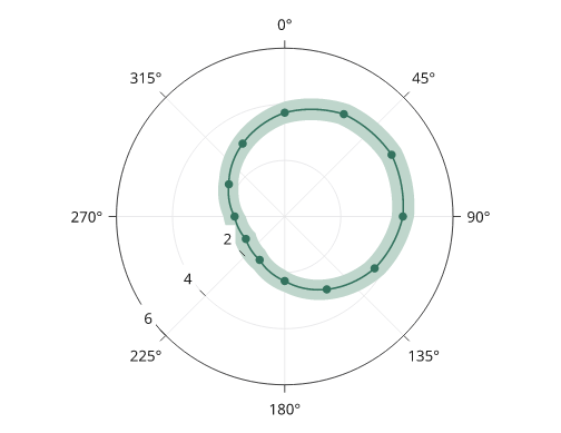
Rendered from the code above.

Rose plots¶

A rose draws radial bars at supplied angles. Heights are radii, so wedge area grows nonlinearly with the value. The optional mean vector below is the count-weighted circular mean of the bin centres; its length represents resultant concentration, not a mean count.

import inklet as i
angles, counts = list(range(0, 360, 45)), [3, 6, 8, 5, 2, 1, 2, 4]
p = i.polar(24, r=(0, 10), zero='up', winding='cw')
p.grid(r_count=2, theta_count=8)
p.rose(counts, at=angles, width=.85, color='#527da8')
p.mean_vector(angles, counts, stroke='#a64736', stroke_width=.6)
p.theta_axis(count=8)
p.r_axis(at=225, count=2)
fig = i.figure(width=80)
fig.add(p.build())
fig.save('rose.svg', 'rose.pdf')

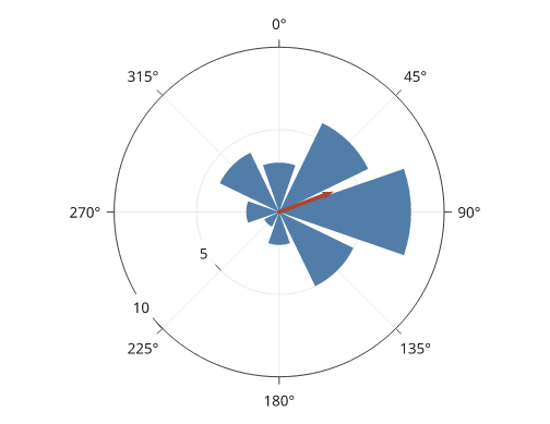
Rendered from the code above.

Radar charts¶

A radar chart places one spoke per category, equally spaced round the turn, and draws each series as a closed polygon through its value on each spoke. radar_grid draws the rings, the spokes and the category names. Rings are polygons by default; shape='circle' draws circles. The panel's theta domain must be a whole turn.

import inklet as i
axes = ['Speed', 'Accuracy', 'Recall', 'Depth', 'Range', 'Stability']
p = i.polar(18, r=(0, 1), zero='up', winding='cw')
p.radar_grid(axes)
p.radar([.8, .6, .9, .4, .7, .5], name='Model A', color='#24698c')
p.radar([.5, .9, .6, .8, .4, .7], name='Model B', color='#b86443')
p.legend(side='bottom')
fig = i.figure(width=80)
fig.add(p.build())
fig.save('radar.svg', 'radar.pdf')

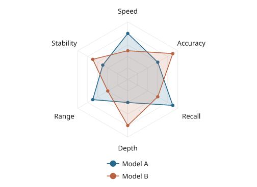
Illustrative scores between 0 and 1. The rings are at 0.2 steps.

radar_grid(values=True) writes ring values up one gap between two spokes, on a paper halo. They are placed when the panel is built, in the gap where the most values keep clear of every series' lines and dots; a value that would touch the data is left out. On a crowded chart only one or two values may fit, so they are off by default; the caption can state the ring steps instead.

Pie and donut charts¶

pie divides the turn in proportion to the values, starting at the start of the theta domain and following the panel's winding. A panel made with hole= draws a donut. Each label is set inside its slice when it fits and outside the rim when it does not. labels= takes 'percent' (default), 'value', None, a format such as '{share:.1%}', a function of (value, share) or one string per slice.

import inklet as i
pie = i.polar(14, zero='up', winding='cw')
pie.pie([54, 28, 12, 4, 2],
        color=['#24698c', '#288675', '#b86443', '#e6b93f', '#b9b8b4'],
        name=['Neurons', 'Glia', 'Vascular', 'Immune', 'Other'])
pie.legend(side='right')
donut = i.polar(14, hole=7, zero='up', winding='cw')
donut.pie([61, 39], color=['#668fb8', '#e6b93f'])
fig = i.figure(width=120)
fig.add(i.row([pie.build(), donut.build()]))
fig.save('pie.svg', 'pie.pdf')

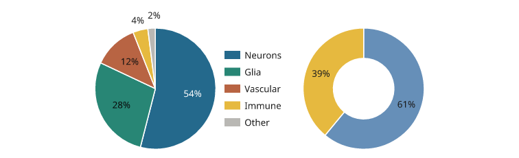
Illustrative shares. The two smallest slices are labelled outside the rim.

An outside label that would overlap another moves out or round the rim to the nearest clear spot. A label that ends up away from its slice gets a hairline leader back to the rim; the pie_labels note lists those slices under leaders.

Pie breakout bars¶

breakout expands one slice, or several adjacent slices, of the pie into a stacked bar beside the disc. Two connector lines run from the rim at the slices' outer edges to the top and bottom of the bar. Without parts, the bar shows the chosen slices as shares of their sum, in their own colours. With parts, it shows the composition of the slice: those values, in color= or in shades of the slice colour. Each part is labelled with its share of the bar; labels that would overlap are moved apart.

Call breakout after pie. The pie turns so the middle of the chosen slices faces the bar, with the first slice uppermost. A zero or winding given to i.polar is kept, so i.polar(11, zero='up', winding='cw') draws the pie as given; then put the chosen slices on the side that faces the bar, or the connectors cross the pie. The pie turns only when nothing else is drawn on the panel before breakout.

Pie labels set outside the rim move out or round the rim, on a leader when they leave their slice, to keep clear of the connectors and the bar. A label that cannot is listed under crossing in the pie's pie_labels note; leave it out (labels= with None for that slice) or pass zero=.

A theta_axis on the panel, drawn before or after breakout, keeps its angle labels off the connectors, the bar and the title. A label that touches one is nudged a little along the rim or outward, or dropped when no nudge clears it; a curved label is dropped. The axis's theta_axis note lists the labels nudged and dropped, as does axis_labels in the pie_breakout note.

import inklet as i
ink, yellow, grey = '#262626', '#e6b93f', '#e4e4e4'
share = i.polar(11)
share.pie([24.8, 1.5, 73.7], color=[ink, yellow, grey],
          labels=['24.8%', None, '73.7%'],
          name=['Isomorphic', 'Dimorphic', 'Noise'])
share.breakout([0, 1], labels='{share:.1%}', title='Without noise')
share.legend(side='bottom')
parts = i.polar(11, hole=5.5)
parts.pie([31, 44, 25], color=['#24698c', '#b9b8b4', '#d9d8d4'])
parts.breakout(0, [58, 27, 10, 5], name=['Type 1', 'Type 2', 'Type 3', 'Type 4'])
parts.legend(side='bottom')
fig = i.figure(width=120)
fig.add(i.row([share.build(), parts.build()], gap=8, align='top'))
fig.save('breakout.svg', 'breakout.pdf')

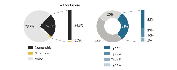
Illustrative shares. Left: the isomorphic and dimorphic slices as shares of their sum. Right: one donut slice divided into four parts.

Next steps¶

Compare plot types, configure axes and scales, or arrange several panels. For exact options, see the API.