Advanced plot layout¶

Control grouped categories, external insets and dense scatter in composite figures such as the twenty-panel stress test.

The examples below build Panel objects directly to show layout controls. They are one sequence: run the imports and first block, then later blocks in order. To export a finished panel, add it to i.document(...) and call save; Panel.build() alone returns an in-memory diagram.

For manuscript figures, keep panel letters, axes, units, scale bars, legends and necessary annotations in the artwork. Put the figure title, panel descriptions, methods and attribution in the manuscript caption. Avoid embedding a suptitle or paragraphs of explanatory prose in the figure. Presentation and teaching figures can use headings when they help the audience.

The microscopy intensity example exports separate caption.tex and caption.txt files alongside its SVG/PDF/PNG artwork.

import inklet

categories = inklet.grouped_band(
    [["All"], ["Binding", "Catalysis"]], gap=1, reverse=True,
)
p = inklet.panel(60, 40, x=(0, 1), y=categories)
p.bars(["All", "Binding", "Catalysis"], [.8, .5, .7], orient="h",
       bar_colors={"All": "#888888", "Binding": "#0053d6", "Catalysis": "#55caf9"},
       stroke="none")
p.axes()

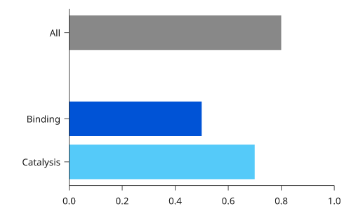
Rendered from the code above.

bar_colors colours individual bars in a single series. A mapping preserves category colours when the input is reordered or filtered; a sequence follows input order. color continues to colour multiple series. Use a separate categorical legend when each bar has its own colour. grouped_band takes ordered groups or a mapping of group names to categories. gap is extra spacing in units of a category step. Group names specify organization; they do not automatically add heading labels.

p = inklet.panel(70, 50, x=(0, 100), y=(0, 100), clip=True)
p.scatter([(20, 30), (90, 94)], raster=True, dpi=300, name="Observations")
p.line([(0, 0), (100, 100)])
p.axes(x="Predicted", y="Observed")
zoom = inklet.panel(30, 25, x=(80, 100), y=(80, 100), clip=True)
zoom.scatter([(90, 94)])
zoom.axes()
p.inset(zoom, side="right", width=None, pad=3,
        zoom=(80, 100, 80, 100), plate=False)

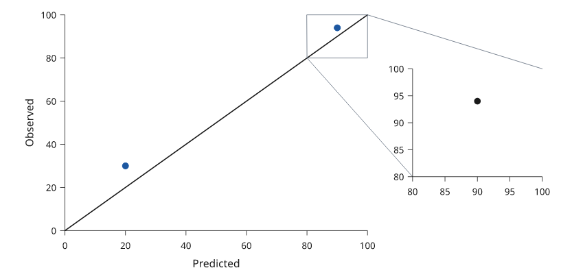
Rendered from the code above.

External inset placement uses the completed parent and child at build time, so axes and labels may be added after inset(). side accepts left, right, top or bottom; align accepts start, center or end and aligns plot areas. width=None preserves the child's physical dimensions and typography. Changes to either panel invalidate the external inset layout; repeated unchanged builds remain cached. Translating or scaling the resulting composition keeps its connectors together. Cyclic inset relationships are rejected.

Rasterization requires inklet[images] (Pillow). Only the requested scatter layer becomes a PNG; axes, legends and other marks remain vector. DPI describes the layer at its authored physical size; scaling the complete figure changes its effective print resolution. Group opacity is applied once after marker compositing. The raster path supports standard markers, solid outlines and clipping, with a 16-million-pixel output limit. Rasterization can increase PDF size or build time; compare exports for the intended density and print size. Matrix rasterization uses the standard-library encoder; see Matrices for its options.

p = inklet.panel(60, 40, x=(0, 2), y=(0, 5))
p.stackarea([0, 1, 2], [[1, 2, 1], [2, 1, 2]], baseline=.5,
            color=["#0053d6", "#55caf9"], name=["A", "B"], stroke="none")
p.axes()
p.legend()

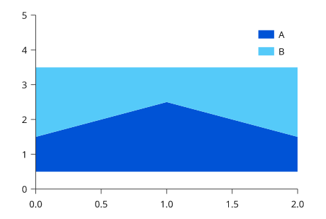
Rendered from the code above.

stackarea accepts series-major, finite, nonnegative values. The baseline may be a finite scalar or a value per x-coordinate. Signed stacked areas require explicitly calculated fill_between bands. Verify that each series uses the same x coordinates and units. A nonzero baseline is useful for a local comparison, but state it in the caption.

Explicit stroke and stroke_width now take precedence over bar and histogram defaults. box(radius=0) keeps square corners under a rounded theme. Explicit tick lists retain the existing thinning default, but omitted labels now trigger a warning: use thin=False to preserve all labels or thin=True to permit thinning explicitly.

Shared category definitions¶

Define category colours and order once. Subsets retain that order and their original colours; empty groups disappear. Display labels travel with the scale.

cats = inklet.categories(
    {'control': '#527da8', 'drug_a': '#cb7853', 'drug_b': '#76a071'},
    labels={'control': 'Control', 'drug_a': 'Drug A', 'drug_b': 'Drug B'},
    groups={'Reference': ['control'], 'Treatment': ['drug_a', 'drug_b']},
)
selected = cats.subset(['drug_b', 'control'])
p = inklet.panel(45, 30, x=(0, 10), y=selected.scale(reverse=True))
p.bars(['control', 'drug_b'], [4, 8], orient='h', bar_colors=selected)
p.axes()
selected.group_labels(p, side='left')  # Add after axes for clearance.
p.legend(side='right', markup=False)

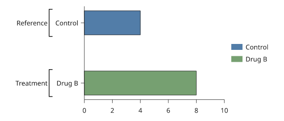
Rendered from the code above.

bar_colors=selected records category legend entries for the supplied bars. For other mark types, use selected[key] for colour and selected.legend_entries with legend(entries=...). Group definitions must partition the category order into consecutive, non-empty groups. After filtering, inspect the resulting order and labels before exporting: an empty group disappears and a reordered subset keeps the shared category order.