

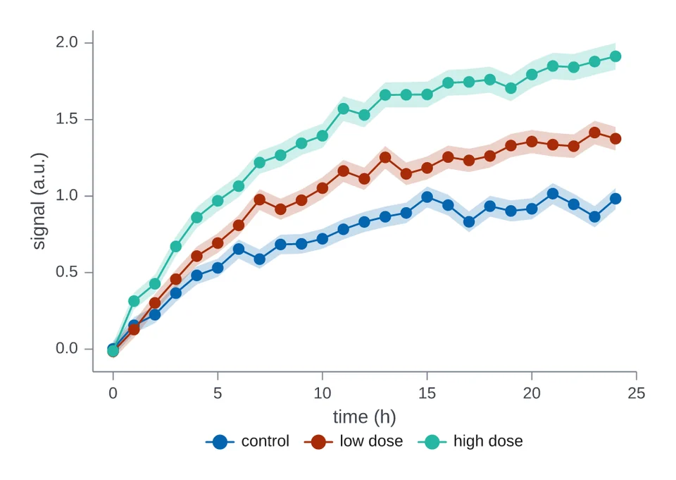
 Lines with an error bandThree curves with standard-error bands, one per condition.
Chart gallery
Every one-call chart type, drawn from simulated data. Each card shows a chart;
selecting it opens the section below with the code that drew it and the
full-size figure. The examples assume import inklet as i. df is a table of
simulated measurements, and each figure names its columns. Options such as
width, palette and legend are described in Charts in one call.
Lines and trends
Series followed along an axis, with their bands and right-hand scales.
Lines with an error bandThree curves with standard-error bands, one per condition.
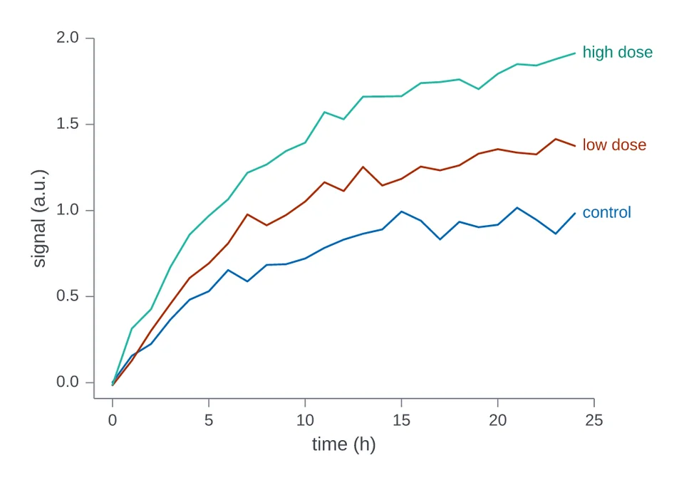 Names at the line endsThe same curves, named where each line ends.
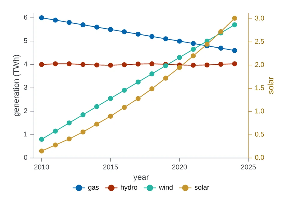 Lines on a right-hand axisSolar on a right-hand axis beside three sources on the left.
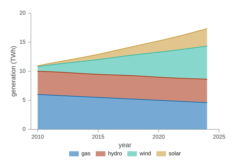 Stacked areasFour sources stacked over fifteen years.
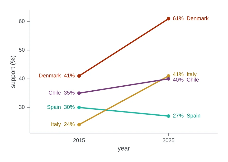 Slope chartEach country's support in two years, joined by a line.
Relationships
Points against points, with fitted lines.
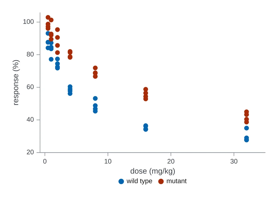 Scatter with groupsPercent response against dose for two strains.
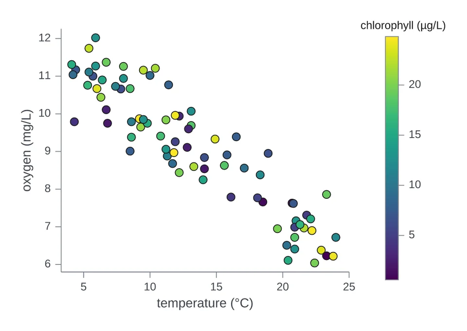 Scatter coloured by a numberPoints coloured by a numeric column, with a colour bar.
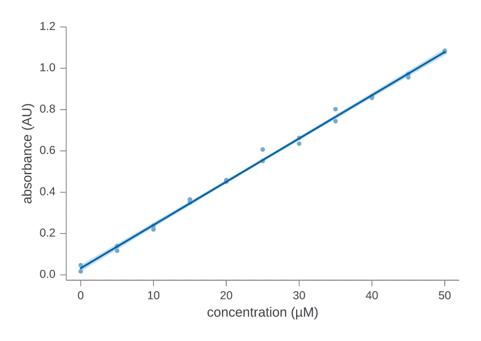 Regression with a confidence bandA fitted line with its 95 per cent confidence band.
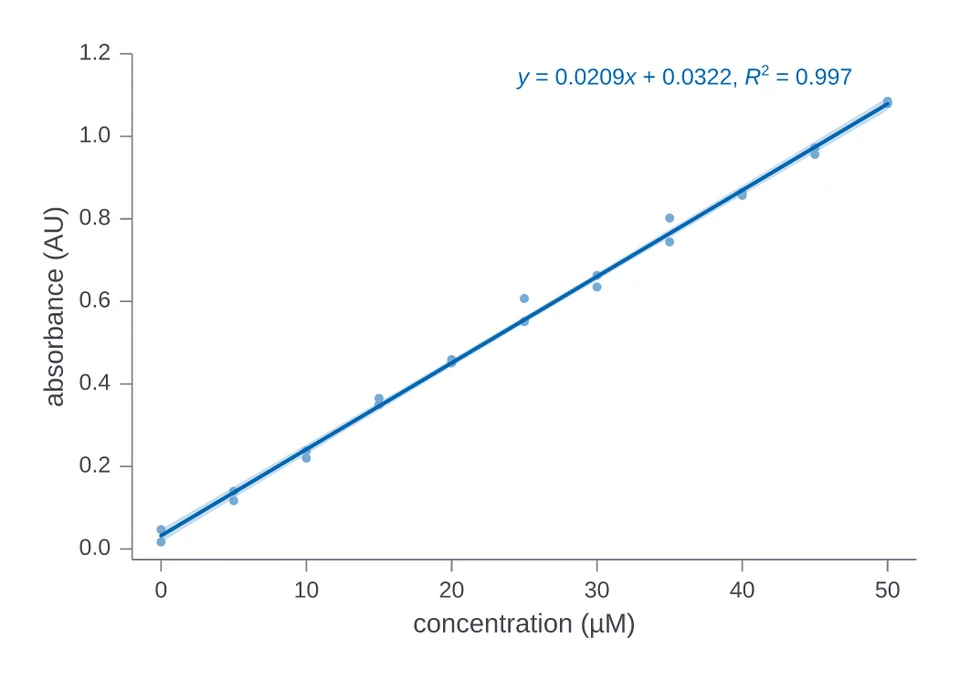 Regression with its equationThe same fit, with its equation written on the plot.
Distributions
The spread of values, as histograms, curves and dots.
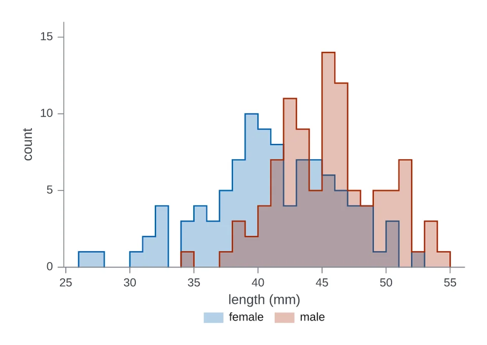 Overlaid histogramsOverlaid histograms of body length by sex.
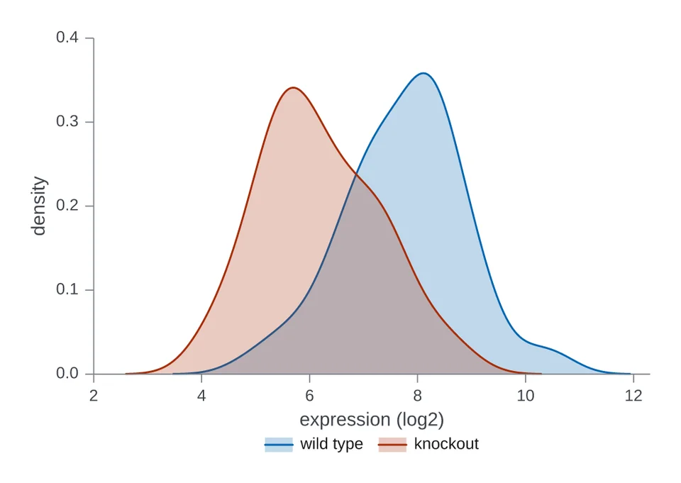 Filled density curvesSmoothed density curves of expression for two genotypes.
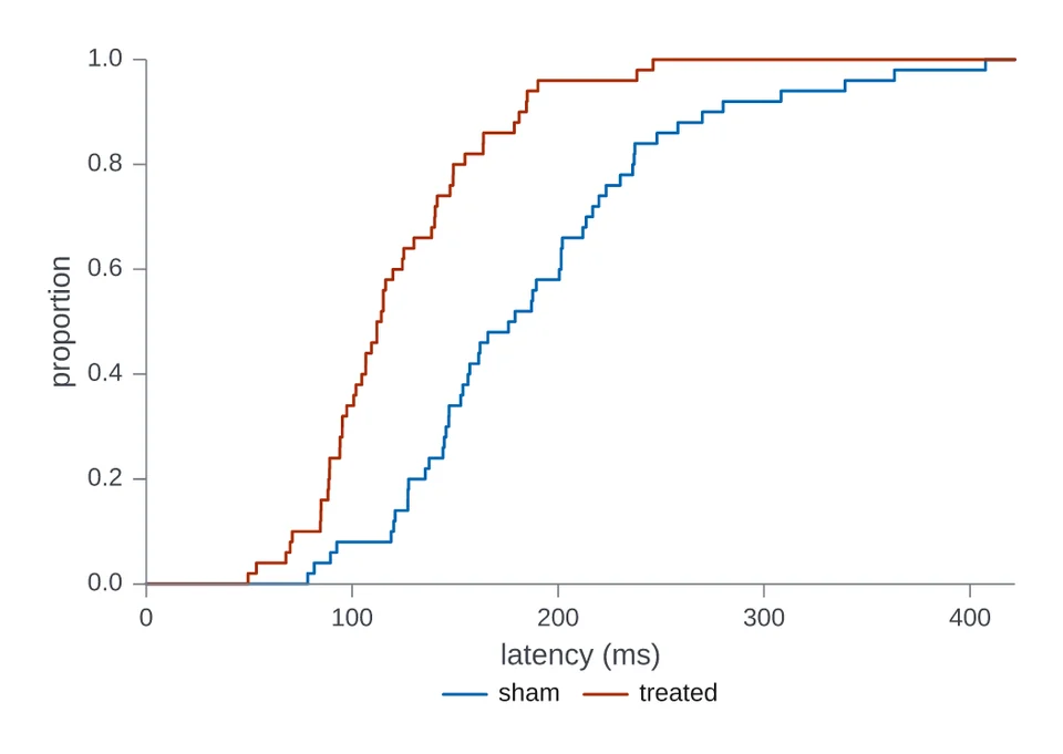 Cumulative distributionsCumulative proportion of latency for two groups.
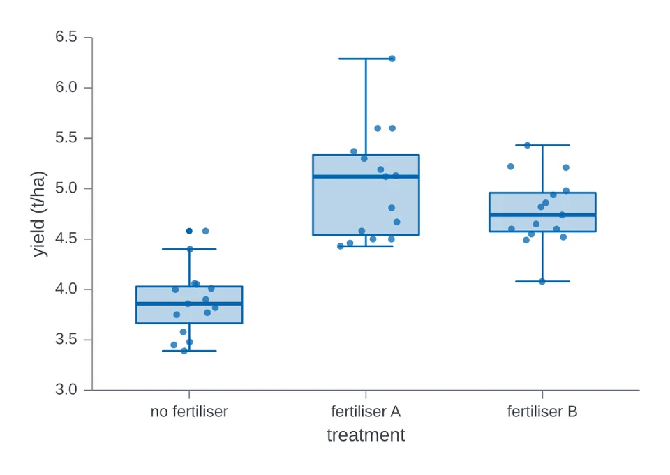 Box plots with pointsBox plots of crop yield, with each plot as a dot.
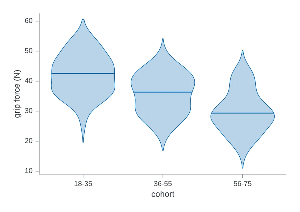 ViolinsViolins of grip force across three age cohorts.
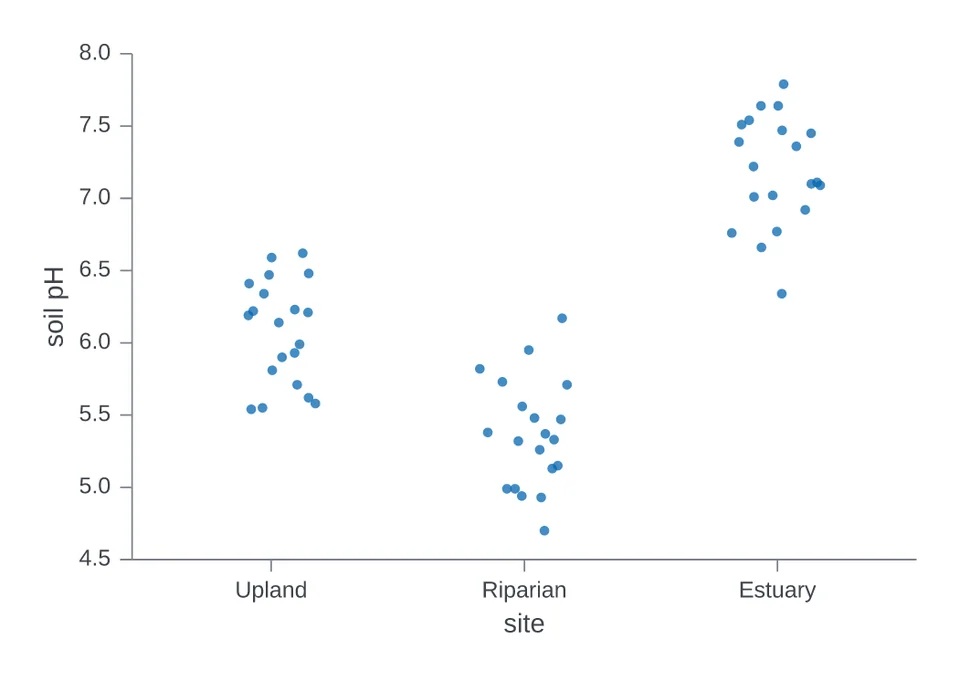 Strip plotJittered dots of soil pH at three sites.
Categories and shares
Bars, dots and wedges for counts and totals.
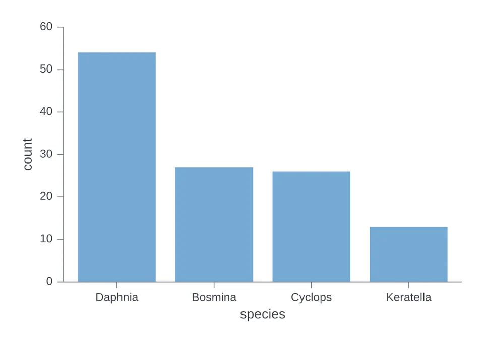 Bars counting rowsBars counting specimens in each species.
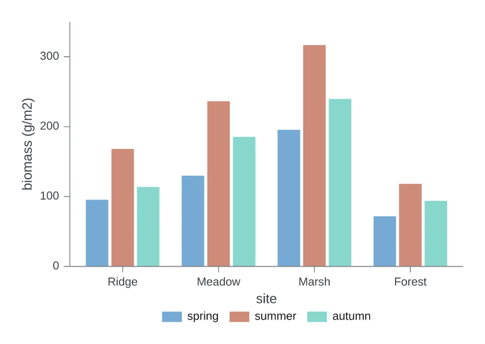 Grouped barsBiomass at four sites, with bars side by side by season.
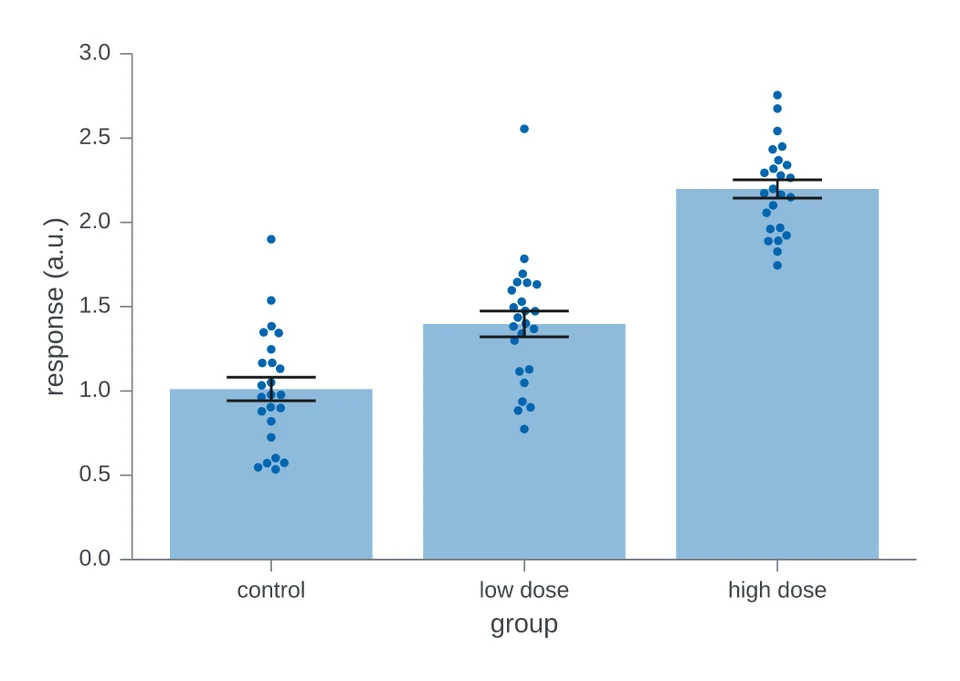 Mean bars with error bars and pointsMean response with error bars and a dot for each animal.
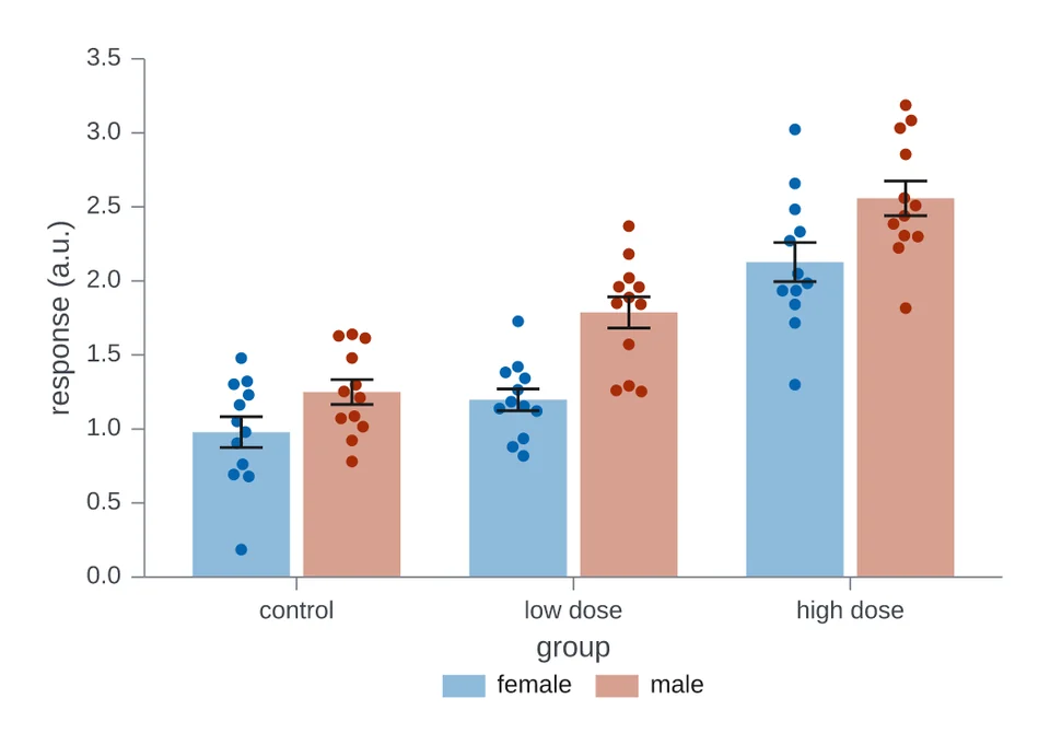 Grouped mean bars with error bars and pointsMean response by group, one bar per sex, with error bars and dots.
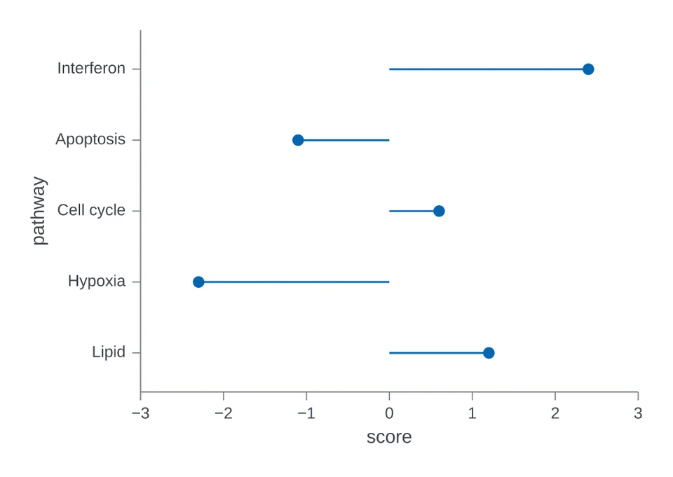 Lollipop chartPathway scores as dots on stems from zero.
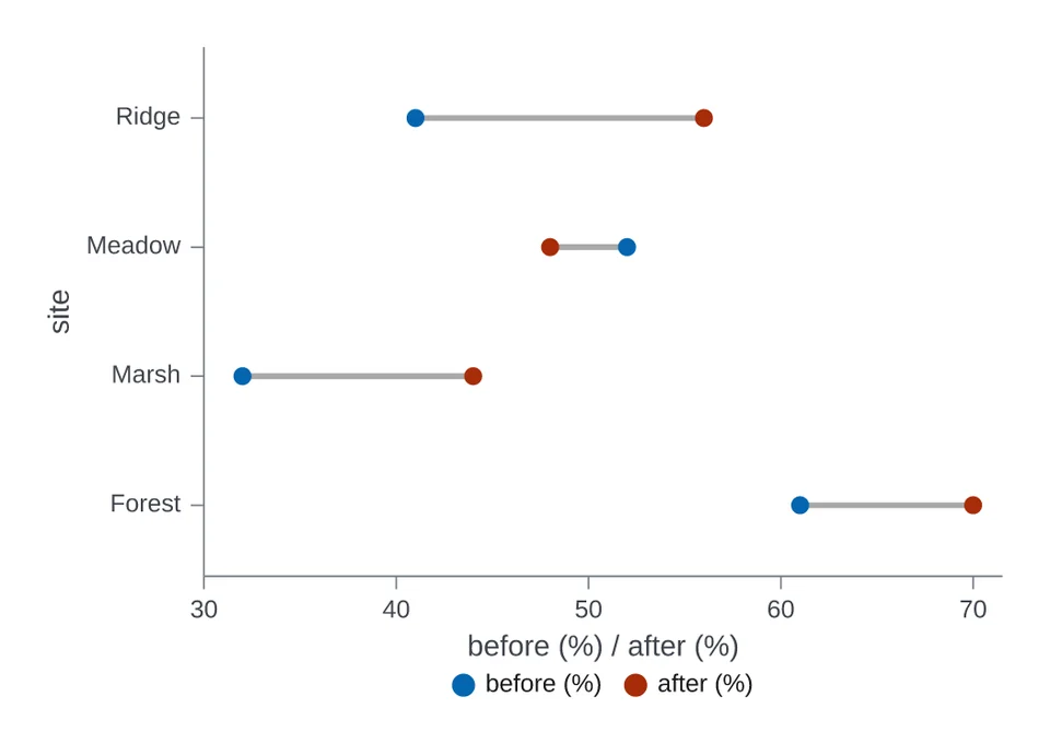 Dumbbell chartSoil moisture before and after a dry season, at four sites.
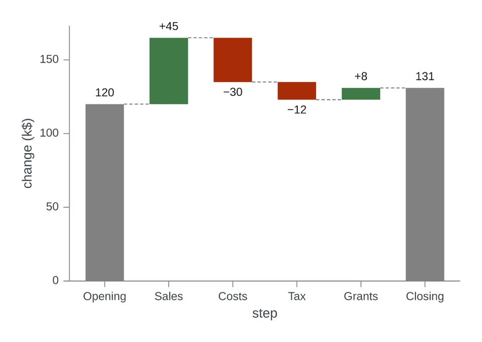 Waterfall chartA budget from its opening balance to its closing balance.
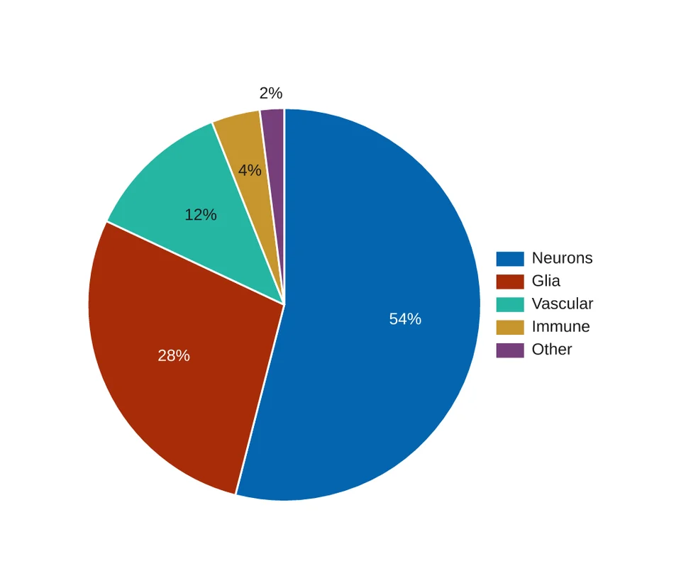 Pie chartCell types in one tissue sample as a pie.
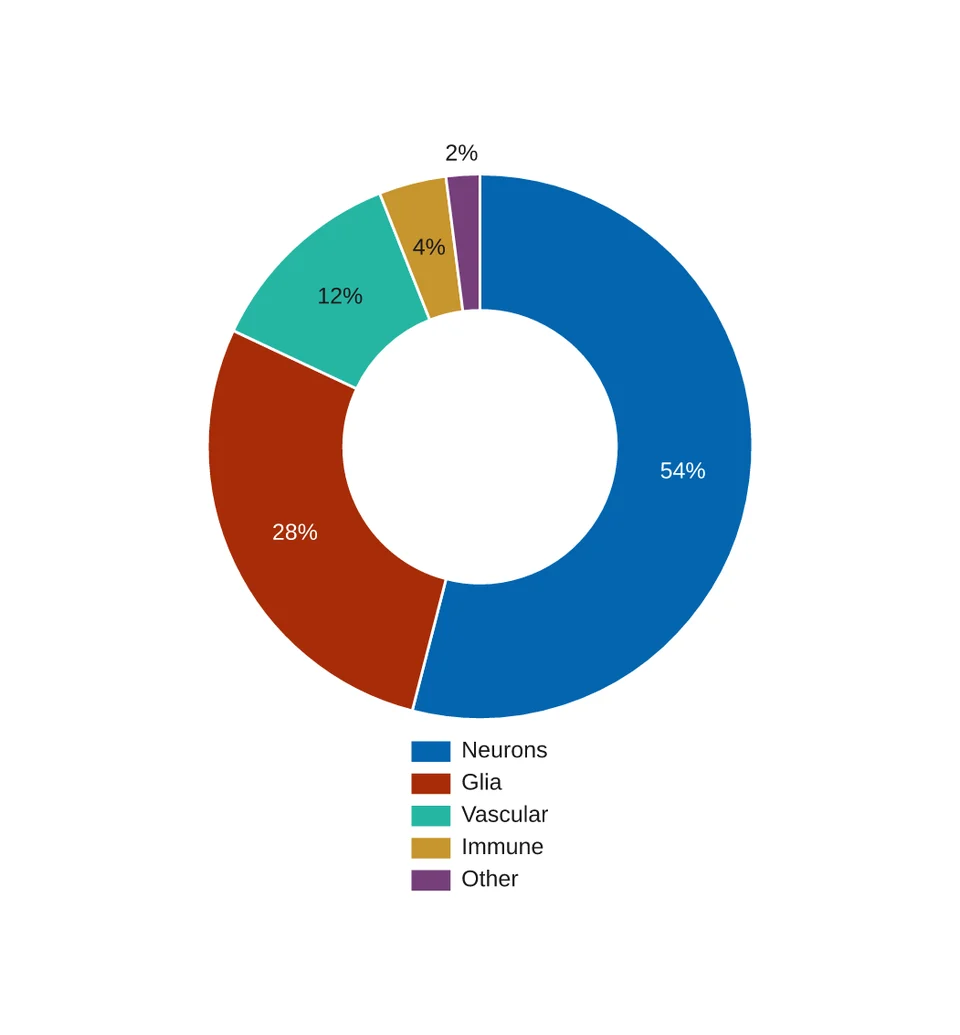 Donut chartThe same cell types as a donut.
Matrices
Values in a grid of coloured cells.
Studies and survival
Statistics from experiments, trials and cohorts.
Panels
Several charts in one figure, with shared axes or lettered panels.
Lines and trends
Series followed along an axis, with their bands and right-hand scales.
Lines with an error band
df has condition, time (h), signal (a.u.) and se (a.u.). The band spans one se (a.u.) either side of each point.
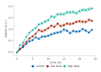
chart = i.line(df, x='time (h)', y='signal (a.u.)', color='condition',
               error_y='se (a.u.)', markers=True)
Names at the line ends
df is the growth table from the first example.
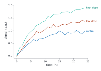
chart = i.line(df, x='time (h)', y='signal (a.u.)', color='condition',
               legend='direct')
Lines on a right-hand axis
df is the generation table from the stacked-area example. secondary_y= puts the named series on a right-hand axis with its own scale.
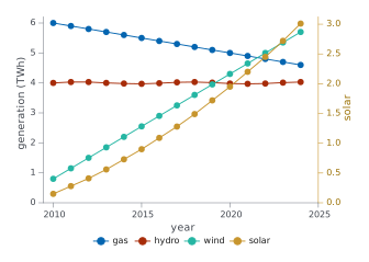
chart = i.line(df, x='year', y='generation (TWh)', color='source',
               secondary_y=['solar'], markers=True)
Stacked areas
df has year, source and generation (TWh). Areas stack unless stacked=False.
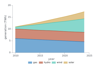
chart = i.area(df, x='year', y='generation (TWh)', color='source')
Slope chart
df has year, country and support (%): two time points per country. format= writes the values as percentages.
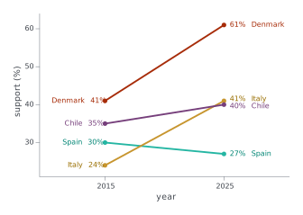
chart = i.slope(df, x='year', y='support (%)', group='country', format='{:.0f}%')
Relationships
Points against points, with fitted lines.
Scatter with groups
df has strain, dose (mg/kg) and response (%).
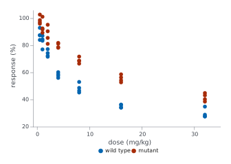
chart = i.scatter(df, x='dose (mg/kg)', y='response (%)', color='strain')
Scatter coloured by a number
df has temperature (°C), oxygen (mg/L) and chlorophyll (µg/L). A numeric color column with many values is drawn as a ramp.
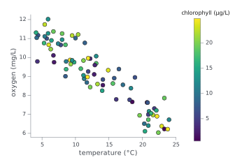
chart = i.scatter(df, x='temperature (°C)', y='oxygen (mg/L)',
                  color='chlorophyll (µg/L)')
Regression with a confidence band
df has concentration (µM) and absorbance (AU), two readings per standard.
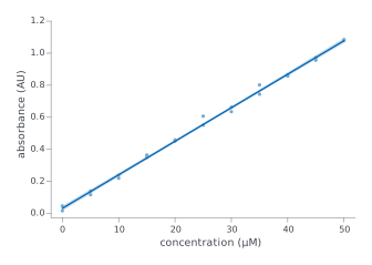
chart = i.regression(df, x='concentration (µM)', y='absorbance (AU)')
Regression with its equation
df is the calibration table from the regression example. equation=True writes the fitted line on the plot.
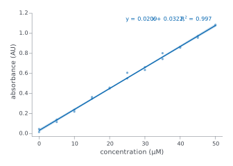
chart = i.regression(df, x='concentration (µM)', y='absorbance (AU)', equation=True)
Distributions
The spread of values, as histograms, curves and dots.
Overlaid histograms
df has sex and length (mm), one row per specimen.
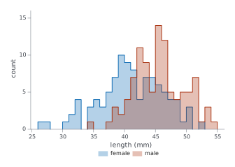
chart = i.hist(df, x='length (mm)', color='sex', bins=20)
Filled density curves
df has genotype and expression (log2), 80 samples per genotype.
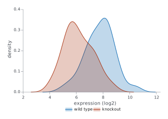
chart = i.kde(df, x='expression (log2)', color='genotype', fill=True)
Cumulative distributions
df has group and latency (ms), 50 animals per group.
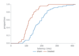
chart = i.ecdf(df, x='latency (ms)', color='group')
Box plots with points
df has treatment and yield (t/ha), 15 plots per treatment.
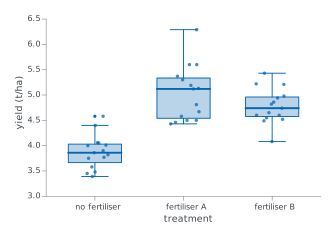
chart = i.boxplot(df, x='treatment', y='yield (t/ha)', points=True)
Violins
df has cohort and grip force (N), 40 people per cohort.
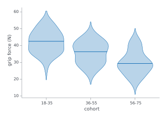
chart = i.violin(df, x='cohort', y='grip force (N)')
Strip plot
df has site and soil pH.
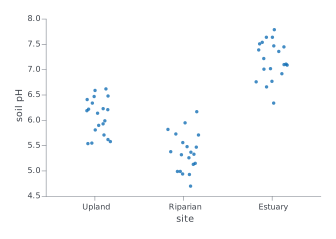
chart = i.strip(df, x='site', y='soil pH')
Categories and shares
Bars, dots and wedges for counts and totals.
Bars counting rows
df has one row per specimen in a species column. Without y, a bar counts its rows.
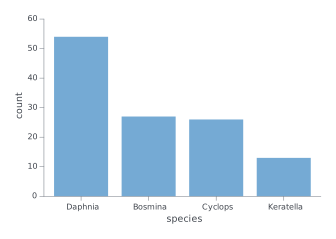
chart = i.bar(df, x='species')
Grouped bars
df has site, season and biomass (g/m2), one row per site and season.
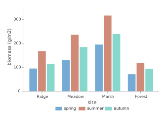
chart = i.bar(df, x='site', y='biomass (g/m2)', color='season')
Mean bars with error bars and points
df has group and response (a.u.), one row per animal. agg= takes the mean of each group, and error_y= takes its standard error.
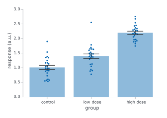
chart = i.bar(df, x='group', y='response (a.u.)', agg='mean',
              error_y='sem', points=True)
Grouped mean bars with error bars and points
df has group, sex and response (a.u.), one row per animal. color= puts the bars side by side, and agg=, error_y= and points= work as they do for a single series.
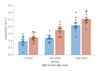
chart = i.bar(df, x='group', y='response (a.u.)', color='sex', agg='mean',
              error_y='sem', points=True)
Lollipop chart
df has pathway and score, one row per pathway. orient='h' lays the stems across the page.
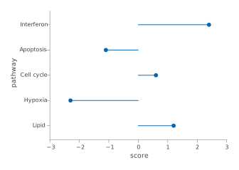
chart = i.lollipop(df, x='pathway', y='score', orient='h')
Dumbbell chart
df has site, before (%) and after (%), one row per site. x= names the two value columns.
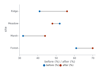
chart = i.dumbbell(df, y='site', x=['before (%)', 'after (%)'])
Waterfall chart
df has step and change (k$). The two totals= steps stand from zero; a missing change on a total shows the running total.
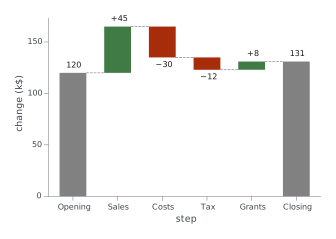
chart = i.waterfall(df, x='step', y='change (k$)', totals=['Opening', 'Closing'])
Pie chart
df has cell type and cells (n), one row per type. The slices are sized by values=, labelled with their shares, and keyed by names=.
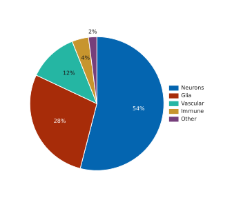
chart = i.pie(df, names='cell type', values='cells (n)')
Donut chart
df is the cell-type table from the pie chart. hole=0.5 leaves a hole half the radius of the disc.
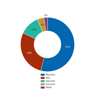
chart = i.pie(df, names='cell type', values='cells (n)', hole=0.5, legend='bottom')
Matrices
Values in a grid of coloured cells.
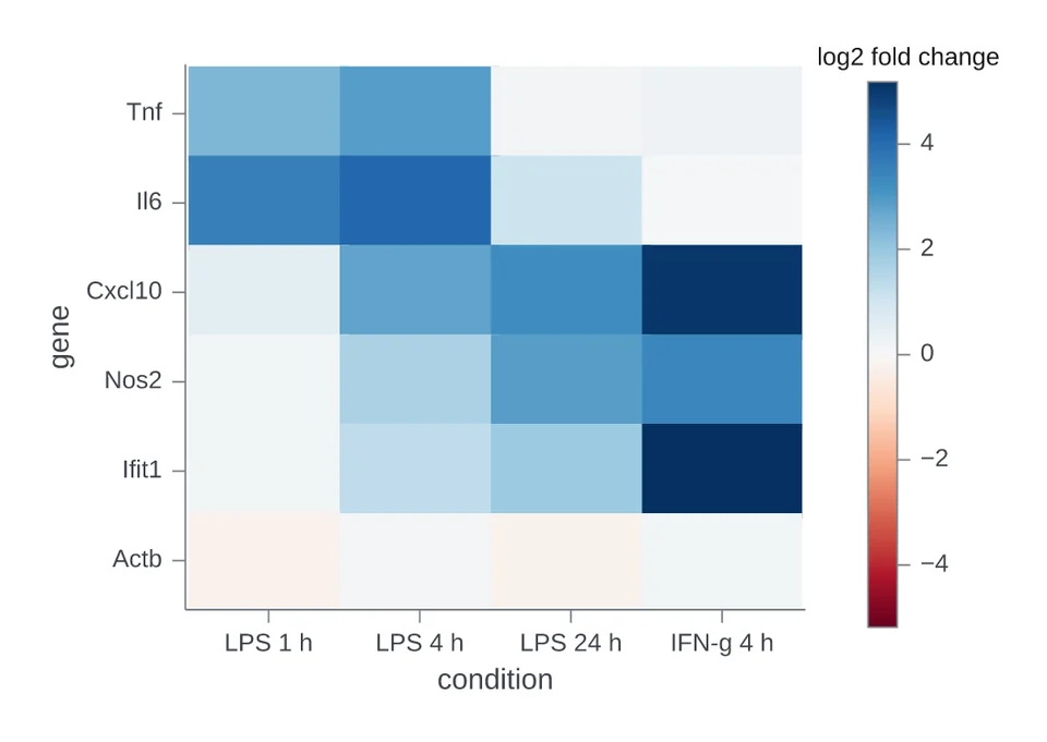
Heatmap with a diverging colour bar
df is a long table with gene, condition and log2 fold change. A diverging palette= with center=0 puts zero at the middle of the colour bar.
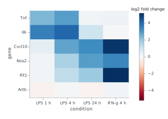
chart = i.heatmap(df, x='condition', y='gene', z='log2 fold change',
                  palette='rdbu', center=0)
Studies and survival
Statistics from experiments, trials and cohorts.
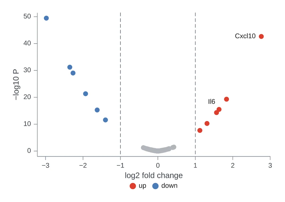
Volcano plot
df has one row per gene: log2 fold change, a raw p-value and an adjusted fdr. q= classes each point by its adjusted p-value, and highlight= names the genes to label.
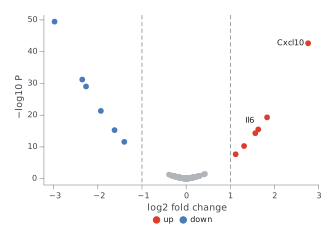
chart = i.volcano(df, x='log2 fold change', y='p-value', label='gene', q='fdr',
                  highlight=['Il6', 'Cxcl10'])
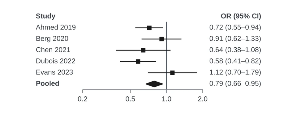
Forest plot
df has study, odds ratio, lower and upper, one row per study. summary= draws a flagged row as a diamond, and right= lists the text beside the plot: here the estimate with its interval.
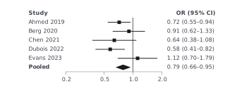
chart = i.quick.forest(df, label='study', estimate='odds ratio', lower='lower',
                       upper='upper', summary='pooled', log=True, measure='OR',
                       right=['ci'])
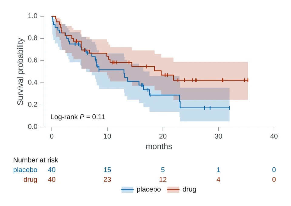
Survival curves
df has arm, months and died. died is 1 where the patient died and 0 where follow-up ended first, which is a censored observation.
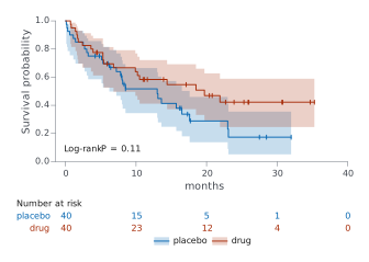
chart = i.survival(df, time='months', event='died', color='arm')
Panels
Several charts in one figure, with shared axes or lettered panels.
Facet panels
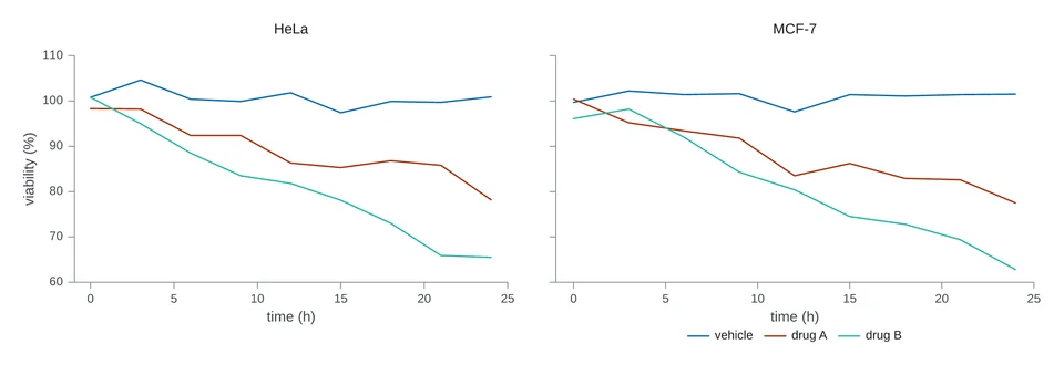
df has cell line, drug, time (h) and viability (%). facet_col= makes one panel per value of a column.
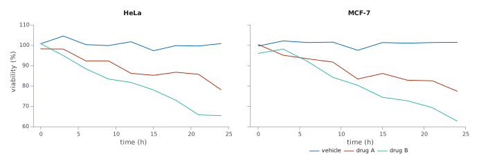
chart = i.line(df, x='time (h)', y='viability (%)', color='drug',
               facet_col='cell line')
Combined panels
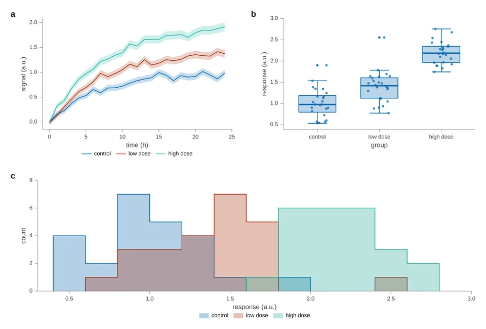
df is the growth table, and outcomes is the response table. | places panels side by side and / stacks them.
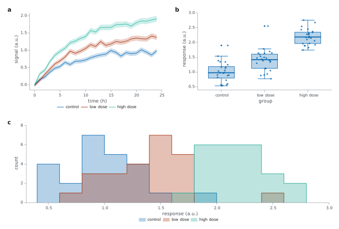
trace = i.line(df, x='time (h)', y='signal (a.u.)', color='condition',
               error_y='se (a.u.)')
spread = i.boxplot(outcomes, x='group', y='response (a.u.)', points=True)
chart = (trace | spread) / i.hist(outcomes, x='response (a.u.)', color='group', bins=14)