Complete regional report¶

Experimental: the API may change.

Build a six-panel offline report with a real map, monthly histories, an empirical distribution and three group comparisons. Select a country, filter a group, save and reopen the view, replace the input table, and export the selected result at 210 mm and 160 mm.

These are opt-in experimental APIs under inklet.experimental.browser.

Open the interactive report · Complete Python recipe · 160 mm version

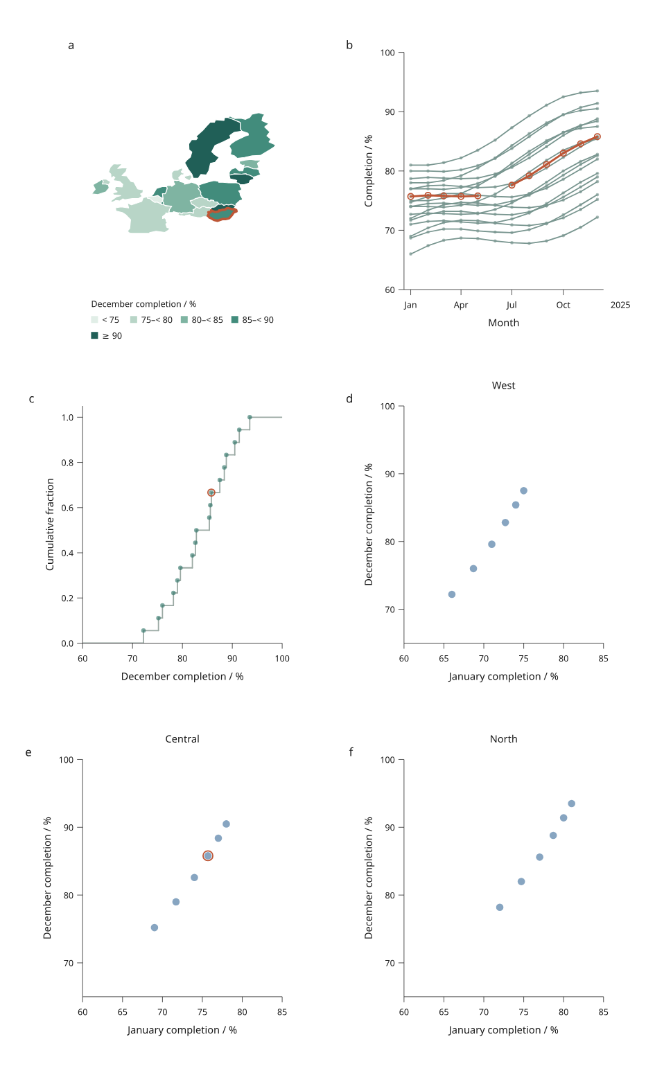
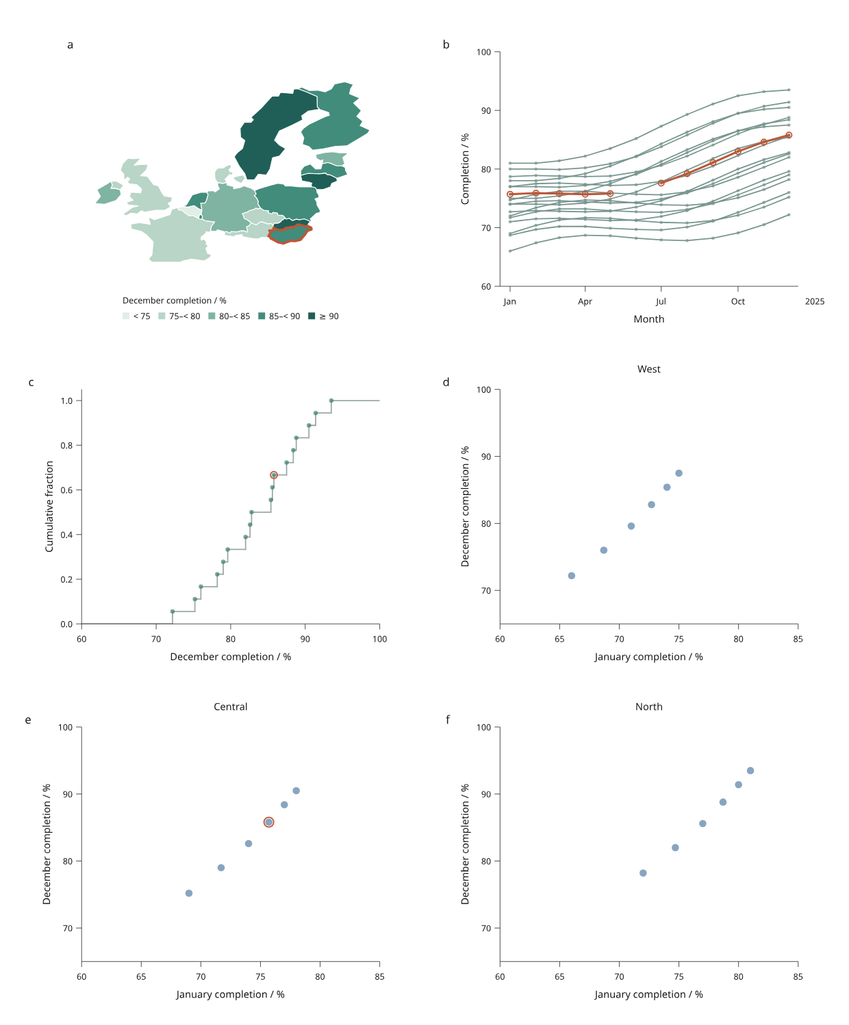
The boundaries are real: 18 country/map units from the pinned, public-domain Natural Earth source. The monthly completion rates are invented measurements, not observations about these countries. Mark Marosi created the simulation as MIT material. The West, Central and North groups are authored for this example. Other countries are omitted; white space on the map does not mean zero completion.

Panel a shows December completion, b shows monthly histories, c shows the fixed December reference distribution, and d–f compare January with December within each group. Orange highlights identify the selected country. Hungary has a missing June sample; the line stops on either side of that gap. Panel labels and category names stay inside the figure; explanatory text belongs in this external caption.

Try the complete workflow¶

python examples/v4/regional_report.py --render --output out/regional-report

HTML, SVG, state JSON, a CSV template, a revision report and provenance are written together. --render also produces PNG and vector PDF at both widths. It needs Chrome/Chromium on PATH and Pillow; PDF conversion uses browser printing, separately from Inklet's native Diagram PDF backend.

1. Open index.html. Hungary is selected initially. Click another country or use its selection button in the data table. Every monthly sample shares that country's identity with the map and other plots.
2. Search for Central. Six countries remain visible. The other category panels retain their axes, and the ECDF reference curve retains all 18 source countries. Filtering hides observations; it does not recalculate statistics.
3. Choose Save view. Reopen that JSON with Open saved view, or reproduce it in Python using the command below.
4. Expand Data revision and switch to the revised table. Hungary's December value changes by 2.5 percentage points; Estonia is removed. If Estonia was selected or explicitly visible, choose the drop policy to remove that ID.
5. Save the revised state. Reconstruct it with --revised --state. The outputs at both physical widths retain the selected and visible country IDs.

# Reopen an original state, preserving its exact viewport in figure.svg.
python examples/v4/regional_report.py --state /path/to/view.json --render --output out/reopened

# Reopen a state saved after switching to the revised table.
python examples/v4/regional_report.py --revised --state /path/to/revised-view.json --render --output out/revised

# Apply an ORIGINAL state to the replacement table, reconciling removed IDs.
python examples/v4/regional_report.py --revised --rebase-state /path/to/view.json --missing drop --render --output out/rebased

figure.svg exactly reconstructs the saved viewport. figure-210mm.svg and figure-160mm.svg recompile the complete page at their named widths and reset the viewport. Their accompanying view-210mm.json and view-160mm.json record those distinct scenes. Browser zoom changes the viewport without remeasuring text or layout. Physical-width exports recompile the layout while retaining authored text and mark sizes.

One series per entity¶

SeriesView uses a wide table: one row per country, with one numeric column per authored sample. It makes that relationship explicit without duplicating country polygons or assigning observation IDs to country boundaries.

from inklet.experimental.browser import BrowserFigure, SeriesView, TimeAxis
from inklet.selection import KeyedTable

table = KeyedTable("countries", {
    "id": ["HUN", "AUT"],
    "jan": [75.7, 69.0], "feb": [75.9, None], "mar": [75.8, 71.3],
})
figure = BrowserFigure(table, [
    SeriesView("history", [("2025-01-01", "jan"),
                           ("2025-02-01", "feb"),
                           ("2025-03-01", "mar")],
               TimeAxis(("2024-12-20", "2025-03-12")), (60, 100),
               x_label="Month", y_label="Completion / %"),
])

Samples are explicit (position, column) pairs. Positions must strictly increase, even with a reversed axis domain; duplicate positions and repeated columns are rejected. Positions can be finite numbers, calendar dates or UTC instants with an explicit TimeAxis. Values must be numeric or None.

A null sample breaks the line. Markers preserve isolated measurements. Optional max_gap_seconds suppresses connections across excessive temporal intervals. radius_mm and line_width_mm control physical mark sizes. FacetView can repeat series over explicit groups, including empty groups.

Clicking a line selects its country; hover reports the nearer endpoint's sample and value, choosing the later endpoint at an exact tie. The table exposes all sample columns for keyboard access. Filtering hides the entire country's series, while a hidden selection remains saved. Replacing the table rebuilds all series and derived comparisons without changing the old scene.

This model deliberately selects entities. Independently selecting an individual country-month observation or linking multiple tables through many-to-one joins remains future work. Use LineView for a series whose observations themselves are the selectable table rows.

Replace the CSV¶

Edit the exported data.csv, retain its exact headers, then run:

python examples/v4/regional_report.py --csv /path/to/replacement.csv --rebase-state /path/to/view.json --missing drop --render --output out/replacement

Empty monthly cells mean missing values. Percentages must be finite and between 0 and 100; IDs must be unique and from the report's 18-country cohort. Groups must be West, Central or North. January, December and their percentage-point change are derived afresh from the monthly columns. The recipe preserves its fixed axes and color bins; values outside a panel's domain are clipped. Adjust make_views() when a different range is appropriate.

The output records the input file's SHA-256 and the pinned geometry provenance; supplied data is labeled separately from the built-in simulation. CSV replacement runs in Python. The offline page switches only between precompiled alternatives; it does not upload or execute arbitrary data processing.

The regional reference workflow now has executable save/reopen, replacement and resize coverage. Broader joins, recomputed filtered summaries, the engineering and scientific reference projects, and the other 4.0 release gates remain open.

Shared compiled renderer¶

The shared compiled renderer was introduced in 4.0.0.dev3:

python examples/v4/regional_report.py --renderer compiled --render --output out/compiled-regional

The same illustrated report above now runs through the shared compiled-scene executor. Select Hungary, filter the Central group, save the view, switch revisions, and reopen the saved view against its matching revision. The state JSON and Python reconstruction commands are unchanged. --backend canvas, --backend svg, or --backend webgl2 explicitly choose execution; the compiled recipe defaults to auto, with reported Canvas fallback when hardware WebGL is unavailable or recognized as software.

In Python, pass renderer='compiled', backend='auto' to BrowserFigure.to_html(). The default renderer remains classic, with its existing SVG/Canvas/hybrid modes. The compiled renderer supports SVG, Canvas, automatic and WebGL2 execution.

Contiguous circle runs use immutable packed records and preserve their row IDs, source paint order, per-mark opacity and physical clipping. Filtering changes candidate indices without replacing those records. Maps, lines and other marks retain native SVG geometry; measured axes and selection outlines stay vector. SVG download and Python SVG/PDF/PNG reconstruction retain the established linked-figure export path. Renderer changes do not change the saved-state digest.

Revision switching prepares the replacement before removing the old renderer, then releases its surfaces, GPU resources and observers. Missing selected or filtered IDs still reject by default; explicit drop produces the same report as Python. Keyboard selection through the source table remains available.

Checks compare the filtered six-panel report against classic SVG at display ratios 1 and 2, and exercise restoration, rejected revisions, explicit removals, export geometry and dense indexed filtering. This is an integration increment: the page still embeds linked interaction geometry alongside packed buffers, picking uses the existing CPU index, and revisions embed complete alternatives. It does not establish a dense-report memory or hardware-speed improvement.

Add --editor for reproducible plot-style editing, with undo/redo and saved overrides that the same recipe can reconstruct.