Relationships between variables¶

Two measured variables per observation call for a different set of plots: densities of many points, fitted lines, agreement between two methods, and grids of every pair. All of them compute in standard-library Python; numpy is not needed.

All values below are illustrative simulated observations. Each snippet can be run independently with core Inklet and writes an SVG and a PDF. The fits and limits are descriptive: no test is run beyond what each section states, and the numbers are there to report, not to replace a statistical analysis.

2D histograms and hexbins¶

When points overlap, count them. hist2d counts points in rectangular bins on continuous axes; hexbin counts them in hexagons that are regular on the page, on log axes too. Both colour each bin by its count through a magma ramp without its palest end, so a bin of one still shows, and colorbar() explains the colours. log=True colours by log count, and min_count leaves sparse bins empty. inklet.plot.histogram2d returns the edges and counts without drawing.

import inklet as i
import random
rng = random.Random(501)
points = []
for _ in range(4000):
    x = rng.gauss(0, 1.1)
    points.append((x, .6 * x + rng.gauss(0, .8)))
hexes = i.plot_spec(x=(-4, 4), y=(-4, 4), height=40)
hexes.hexbin(points, gridsize=22)
hexes.axes(x='Score A', y='Score B')
hexes.colorbar(label='Cells')
cells = i.plot_spec(x=(-4, 4), y=(-4, 4), height=40)
cells.hist2d(points, bins=18)
cells.axes(x='Score A', y='Score B')
cells.colorbar(label='Cells')
doc = i.document(width=130, columns=[1, 1], gap=8)
doc.add('hexes', hexes, row=0, column=0)
doc.add('cells', cells, row=0, column=1)
doc.save('hexbin.svg', 'hexbin.pdf')

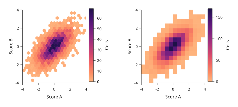
Rendered from the code above: the same 4,000 simulated points counted in hexagons (left) and rectangles (right).

Density-coloured scatter¶

density_scatter keeps every point and colours it by how crowded its neighbourhood is. It estimates the density on the page, so it behaves the same on log axes and follows where the marks actually overlap. The densest points are drawn last. With raster=True the markers are one embedded image, which keeps 100,000 points small in SVG and PDF while the axes and text stay vector. Colours run from 0 to the densest point, so the colour bar reads as relative density.

import inklet as i
import math
import random
rng = random.Random(502)
points = []
for _ in range(100_000):
    u = rng.gauss(0, 1)
    points.append((math.exp(1 + u), math.exp(.5 + .7 * u + .6 * rng.gauss(0, 1))))
p = i.plot_spec(x=i.plot.log((.01, 1000)), y=i.plot.log((.01, 1000)), height=44)
p.density_scatter(points, raster=True, size=.5)
p.axes(x='Intensity A / a.u.', y='Intensity B / a.u.')
p.colorbar(label='Relative density')
doc = i.document(width=80)
doc.add('density', p)
doc.save('density.svg', 'density.pdf')

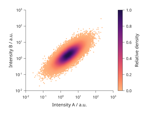
Rendered from the code above: 100,000 simulated log-normal intensities in one embedded image.

2D density contours¶

kde2d draws contours of a Gaussian kernel density. Each contour encloses a share of the estimated probability: levels=(.5, .8, .95) draws the smallest regions that hold 50%, 80% and 95% of it, and levels=5 draws five evenly spaced shares up to 95%. fill=True fills the regions between them from the density ramp, palest outside. The bandwidth per axis follows Scott's rule (sd * n^-1/6) unless given. inklet.plot.kde2d returns the density lattice.

import inklet as i
import random
rng = random.Random(503)
points = []
for _ in range(900):
    centre = (-1.2, -.8) if rng.random() < .55 else (1.4, 1.1)
    points.append((rng.gauss(centre[0], .8), rng.gauss(centre[1], .7)))
lines = i.plot_spec(x=(-4, 4), y=(-4, 4), height=40)
lines.scatter(points, size=.5, color='#bbbbbb')
lines.kde2d(points, levels=(.25, .5, .75, .95))
lines.axes(x='Component 1', y='Component 2')
filled = i.plot_spec(x=(-4, 4), y=(-4, 4), height=40)
filled.kde2d(points, levels=6, fill=True)
filled.axes(x='Component 1', y='Component 2')
doc = i.document(width=110, columns=[1, 1], gap=8)
doc.add('lines', lines, row=0, column=0)
doc.add('filled', filled, row=0, column=1)
doc.save('kde2d.svg', 'kde2d.pdf')

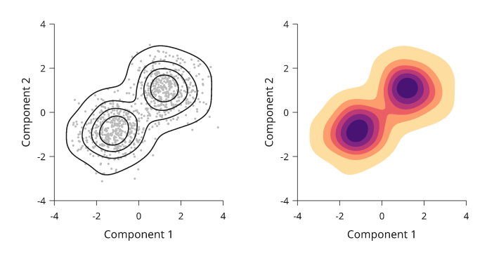
Rendered from the code above. The contours hold 25%, 50%, 75% and 95% of the estimated density of 900 simulated points from two clusters.

Contours of a gridded field¶

contour(x, y, z, ...) draws lines through a field that is already sampled on a grid, such as the counts of a 2D histogram or a simulated surface. z[j][i] is the value at (x[i], y[j]), the same layout as matrix(). Give the values in levels=, or give the shares of the total that the regions should hold in hdr=: hdr=(0.683, 0.954) draws the highest-density regions holding 68.3% and 95.4% of the counts. inklet.plot.mass_levels(z, (0.683, 0.954)) returns the values behind those regions for a grid, without drawing.

import inklet as i
import random
from inklet.plot import histogram2d
rng = random.Random(611)
points = [(rng.gauss(0, 1.1), rng.gauss(0, .8)) for _ in range(1200)]
x_edges, y_edges, counts = histogram2d(points, bins=(16, 16), range=((-3, 3), (-3, 3)))
x = [(a + b) / 2 for a, b in zip(x_edges, x_edges[1:])]
y = [(a + b) / 2 for a, b in zip(y_edges, y_edges[1:])]
p = i.plot_spec(x=(-3, 3), y=(-3, 3), height=60)
p.contour(x, y, counts, hdr=(0.683, 0.954), color=['#24698c', '#b8512e'])
p.axes(x='Component 1', y='Component 2')
doc = i.document(width=110)
doc.add('contours', p)
doc.save('contours.svg', 'contours.pdf')

Contours follow a log axis as the axis bends, and the lines are cut to the plot area unless clip=False. A missing value (None) lies outside every level, so a contour closes round a gap instead of through it. A level outside the range of z draws nothing, and if none is inside it the call fails.

Regression and residuals¶

regression draws the points, a least-squares line and its 95% confidence band for the mean response, from Student's t on n - 2 degrees of freedom. prediction=True shades the wider interval for a new observation instead. method='lowess' draws R's lowess() smoother. The line's node carries a regression note with the slope, intercept, R² and p-value; compute them with inklet.plot.linear_fit, which matches R's lm on the cars data. On a log x axis the fit is of y on log10 x, so the line stays straight. residuals draws what the fit left, against x, with a zero line. smooth=True adds a LOWESS trend.

import inklet as i
from inklet.plot import linear_fit
speed = [4, 4, 7, 7, 8, 9, 10, 10, 10, 11, 11, 12, 12, 12, 12, 13, 13, 13, 13,
         14, 14, 14, 14, 15, 15, 15, 16, 16, 17, 17, 17, 18, 18, 18, 18, 19,
         19, 19, 20, 20, 20, 20, 20, 22, 23, 24, 24, 24, 24, 25]
dist = [2, 10, 4, 22, 16, 10, 18, 26, 34, 17, 28, 14, 20, 24, 28, 26, 34, 34,
        46, 26, 36, 60, 80, 20, 26, 54, 32, 40, 32, 40, 50, 42, 56, 76, 84, 36,
        46, 68, 32, 48, 52, 56, 64, 66, 54, 70, 92, 93, 120, 85]
cars = list(zip(speed, dist))
fit = linear_fit(cars)
line = i.plot_spec(x=(0, 26), y=(-20, 125), height=40)
line.regression(cars)
line.axes(x='Speed / mph', y='Stopping distance / ft')
line.text(1, 110, f'R² = {fit.r2:.2f}', anchor='w')
left = i.plot_spec(x=(0, 26), y=(-40, 50), height=40)
left.residuals(cars, smooth=True)
left.axes(x='Speed / mph', y='Residual / ft')
doc = i.document(width=120, columns=[1, 1], gap=8)
doc.add('fit', line, row=0, column=0)
doc.add('residuals', left, row=0, column=1)
doc.save('regression.svg', 'regression.pdf')

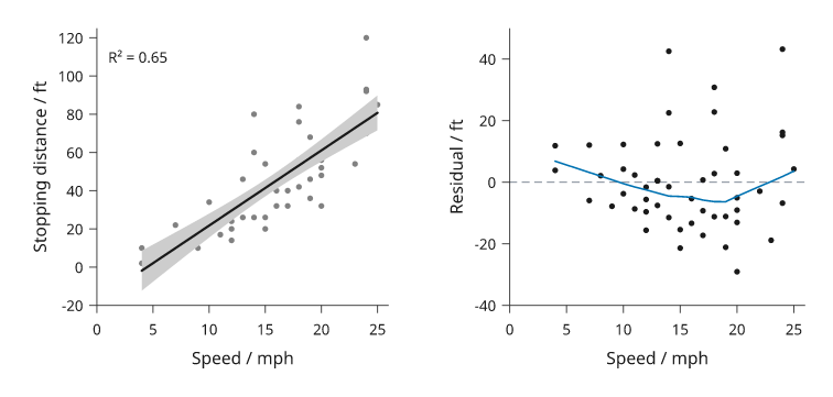
Rendered from R's cars data (Ezekiel, 1930). The residuals widen with speed, which the straight fit does not model.

Bland-Altman agreement¶

bland_altman compares two methods that measure the same subjects. Each pair is drawn at its mean and its difference. A solid line marks the bias (the mean difference) and dashed lines the limits of agreement, bias ± 1.96 SD, with each value set in the right margin clear of the data. confidence=0.95 shades the confidence interval of the bias and of each limit (Bland and Altman, 1986). percent=True plots differences as a percentage of the mean. inklet.plot.bland_altman(a, b) returns the same numbers, which set the y domain.

import inklet as i
import random
from inklet.plot import bland_altman
rng = random.Random(504)
truth = [rng.uniform(60, 180) for _ in range(80)]
meter = [t + rng.gauss(2.5, 4.5) for t in truth]
lab = [t + rng.gauss(0, 3.0) for t in truth]
agreement = bland_altman(meter, lab)
p = i.plot_spec(x=(50, 190), y=(-25, 30), height=40)
p.bland_altman(meter, lab, confidence=.95, format='{:.1f}')
p.axes(x='Mean of methods / mg dl⁻¹', y='Meter − lab / mg dl⁻¹')
doc = i.document(width=90)
doc.add('bland-altman', p)
doc.save('bland-altman.svg', 'bland-altman.pdf')

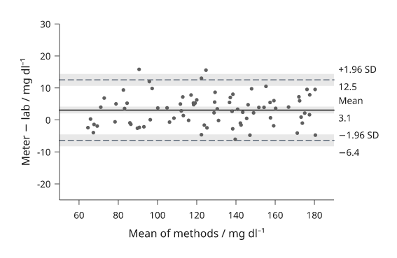
Rendered from the code above: 80 simulated paired glucose readings.

Pair plots¶

inklet.pairplot draws every pair of variables in one aligned grid. Each column shares an x scale and each row a y scale, and only the outer panels write numbers and names. The diagonal shows each variable's distribution. The lower and upper triangles draw 'scatter', 'kde2d', 'hexbin', 'hist2d', 'regression' or nothing. groups= colours observations by label and keys them. The diagonal then shows per-group densities, which overlap more legibly than histograms. corner=True drops the upper triangle. The result is a diagram, so it goes into row, column or a document like a panel.

import inklet as i
import random
rng = random.Random(505)
species, data = [], {'Sepal length': [], 'Sepal width': [], 'Petal length': []}
for name, (a, b, c) in {'setosa': (5.0, 3.4, 1.5), 'versicolor': (5.9, 2.8, 4.3),
                        'virginica': (6.6, 3.0, 5.5)}.items():
    for _ in range(50):
        species.append(name)
        data['Sepal length'].append(rng.gauss(a, .4))
        data['Sepal width'].append(rng.gauss(b, .3))
        data['Petal length'].append(rng.gauss(c, .45))
grid = i.pairplot(data, groups=species, cell=24)
doc = i.document(width=125)
doc.add('pairs', grid)
doc.save('pairs.svg', 'pairs.pdf')

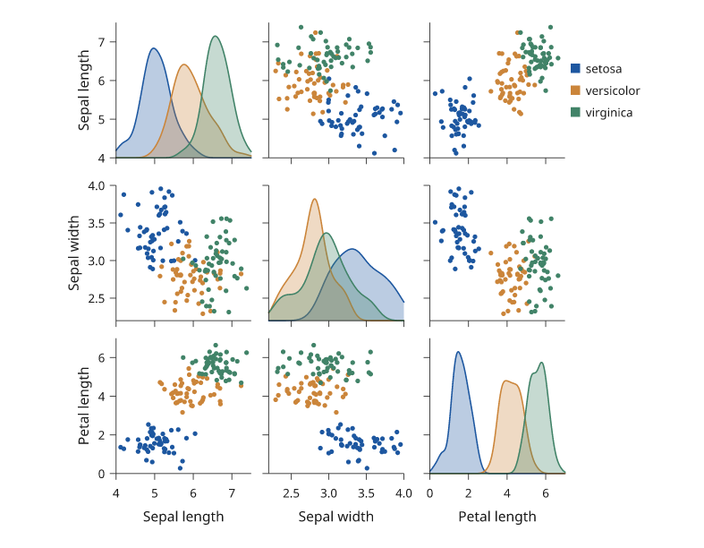
Rendered from the code above: simulated measurements in the spirit of Anderson's iris data, 50 per group.

Joint plots¶

inklet.jointplot draws one pair with both marginal distributions along the top and right edges, on the main panel's own scales. The main panel draws kind ('scatter', 'kde2d', 'hexbin', 'hist2d' or 'regression') and the margins marginal='hist' or 'kde'. width is the main panel's side and ratio its size relative to the margins. The margins carry no count axis, since only their shape is read.

import inklet as i
import random
rng = random.Random(506)
points = []
for _ in range(3000):
    x = rng.gauss(0, 1)
    points.append((x, .55 * x + rng.gauss(0, .85)))
joint = i.jointplot(points, kind='hexbin', marginal='kde', width=46,
                    x_label='Score A', y_label='Score B')
doc = i.document(width=80)
doc.add('joint', joint)
doc.save('joint.svg', 'joint.pdf')

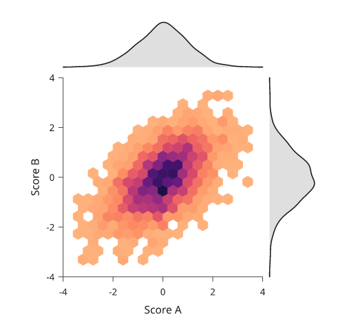
Rendered from the code above.

Next steps¶

See distributions for one variable at a time and uncertainty for supplied intervals. For exact options, see the API.