

On this page
Rendering and layout review
This page records historical engine measurements from named development revisions. Use the current dense data guide and compiled viewer guide for current workflows; the figures below are reproducibility studies, not current performance budgets.
For the next engine architecture increment after dev2, see packed vector markers and shared compiled scenes, including revision reuse and complete-figure measurements.
For the engine changes included in 4.0.0.dev2, see the illustrated transparency and compositing review, including PNG alpha, single-primitive opacity and nested PDF export measurements. The next hatch engine increment shares exact line geometry across SVG/PDF and records the performance and file-size tradeoffs of reusable fills.
Inklet 3.1 improves dense raster plots, repeated-image exports, fixed-component reuse and nested layout. It also fixes a PDF clipping defect: transparency groups now include the full painted stroke and text halo, even when those extend beyond the drawing's layout envelope.
Full-size figure · Executable recipe · LaTeX caption

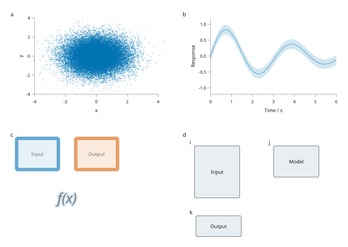
The data are simulated and all artwork is original. Panel a contains 30,000 points; its axes and labels remain vector. Panel b's interval is supplied by the recipe and has no inferred statistical meaning. Panels c and d exercise transparency bounds and unequal fixed-size drawings with panel letters. Descriptions and methods are in the separate caption.
Reproduce the figure
These changes are included in Inklet 3.1. Check out v3.1.0 to reproduce this recipe.
git clone --branch v3.1.0 https://github.com/Mapika/inklet.git
cd inklet
python -m pip install -e '.[render]'
python examples/engine_review.py
This writes SVG, PDF, PNG, text/LaTeX captions and a diagnostic report into
out/engine-review/. There are no external assets or downloads. The example
allows informational diagnostics and rejects errors and warnings.
PDF transparency: before and after
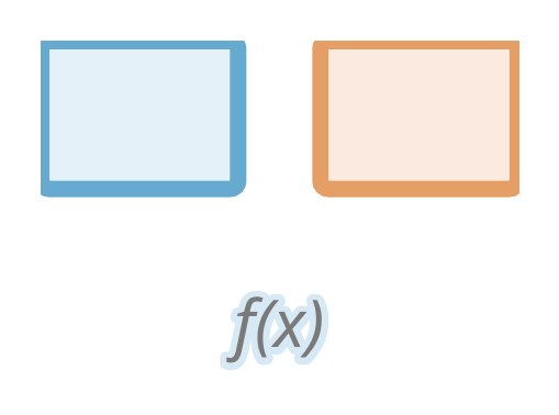
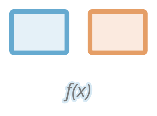
Both images below use the same drawing and Poppler rasterizer. The previous
engine uses commit b07858b; the current engine includes painted bounds.
SVG artwork already contained these strokes. The defect was specific to the
PDF transparency group's clipping rectangle.
Previous PDF: the top and outer sides of the blocks lose part of their strokes.
Current PDF: complete strokes and corners remain visible.
To render this specimen separately, use python examples/engine_review.py
--quality-only. Its SVG and PDF go to out/engine-review/. The same recipe can
run against the previous engine through PYTHONPATH pointing to that checkout's
src directory. Rasterize both PDFs with pdftoppm -r 190 -png -singlefile.
What changed
- Dense scatter: raster plots resolve bounded marker prototypes and paint directly, avoiding a temporary drawing tree for every point. Point order, per-point sizes/colours, clipping and fill/group opacity keep their meanings. All seven marker shapes retain the existing antialiasing and stroke rules. Explicit placement options use the established tree renderer.
- Layout: ordinary track constraints use a direct projection onto their minima; overlapping spans retain the general solver. Plot-margin sharing groups cells by row/column instead of comparing every pair. Fixed factories reuse their results across measurement and resize passes.
- Alignment:
document.add(..., align='nw')and the other compass points place fixed artwork within a cell without scaling. Nested fixed drawings retain the measured space required by their panel letters. - Geometry and styles: copies that only change identity or paint reuse immutable measured geometry. Style inheritance uses a bounded cache. Anchors and annotations on a copy remain separate from the original.
- Exports: repeated images encode and hash once per export. File-backed images are read again for the next export. PDF font subsets omit shaping tables before parsing them, since their glyphs have already been shaped; SVG webfonts retain those tables for viewer-side shaping.
Performance measurements
The benchmark tool runs three complete workloads in fresh Python processes. Each repeat measures compilation, cached compilation, first SVG/PDF export, repeated exports, output size and peak process memory. Imports and recipe construction are outside the timed phases; peak memory includes the whole worker process. Repeated exports must be byte-identical and cached compilation must return the same snapshot.
Previous engine measurements · Development engine measurements
Measurements below use the median of three fresh-process runs on this Linux WSL2 workstation with Python 3.12.3. They are comparisons on this machine, not guarantees for other hardware. Raw reports include each repeat, dependency versions and a source hash. The benchmark raster cloud uses 150 dpi; the review figure above uses 300 dpi.
| Workload / phase | Previous engine | Development engine | Change |
|---|---|---|---|
| 30,000-point raster plot: compile | 15.4891 s | 4.8466 s | 3.20× faster |
| 30,000-point raster plot: peak process memory | 350.7 MiB | 100.1 MiB | 71% lower |
| 64 plots: compile | 0.8878 s | 0.6552 s | 1.35× faster |
| 64 plots: first PDF export | 0.1792 s | 0.0597 s | 3.00× faster |
| 64 plots: first SVG export | 0.1215 s | 0.1779 s | 1.46× slower |
| 64 repeated images: SVG export | 0.0233 s | 0.0025 s | 9.47× faster |
python tools/benchmark_engine.py --output out/engine-after.json
python tools/benchmark_engine.py --source /path/to/previous/inklet \
  --output out/engine-before.json
The ordinary grid's first SVG export can vary independently of its compilation and PDF improvements. Consult the separate phase timings in the raw reports; the engine does not make every export path faster. Pixel output still depends on the selected renderer, fonts and DPI. The existing visual tests use pinned renderer versions and reviewed baselines.
Curve-preserving geometric clipping and explicit painted windows now share resolved clip regions across SVG/PDF, with separate layout and painted bounds. See the clipping review for semantics, limits and measurements.
Core optimization measurements (dev15)
The current core avoids corner/hull construction for rectangle envelopes and
transformed bounds, skips allocation when composing identity transforms, and
reuses theme defaults and contrast choices within a build. These changes apply
to existing drawing APIs. The redundant internal CompositingAnalysis cache was
removed; production exporters already obtain cached bounds and paint counts from
compiled SceneNode objects. Its behavioral tests now exercise those snapshots.
Measurements below use Python 3.12.3 on Linux/WSL2. Core workloads use seven fresh processes; complete figures use five. Baseline and revised runs were sequential, with ordinary garbage collection enabled. Timings exclude imports and recipe setup. These are measured workloads, not universal speedup guarantees.
| Workload | Before | After | Result |
|---|---|---|---|
| 10,000 rectangles: theme, compile, bounds, resolve, revision, SVG | 783 ms | 524 ms | 33% less time |
| 2,000 labels: same operations | 351 ms | 265 ms | 24% less time |
| Complete 64-panel figure: compile | 742 ms | 630 ms | 15% less time |
| Complete 64-panel figure: compile and all measured exports | 995 ms | 941 ms | 5% less time |
| Complete 64-panel figure: peak process RSS | 99.6 MiB | 93.7 MiB | 6% less memory |
| Nested transparency: compile and all measured exports | 303 ms | 305 ms | Essentially unchanged |
Core fixtures retain identical SVG hashes and bounds. Phase timings can move in opposite directions when garbage collection shifts between phases; compare the whole workflow as well as the raw timings. For example, initial SVG export of the 64-panel figure took longer even though the overall cycle improved.
The four changed production files contain nine fewer physical lines in total. The reduction comes from removing a duplicate cache, while retaining explanatory comments and adding explicit fast paths. Tests and the benchmark harness add code.
Run the core benchmark against two source checkouts:
python tools/benchmark_core.py --source /path/to/baseline --repeat 7 --output before.json
python tools/benchmark_core.py --source /path/to/revised --repeat 7 --output after.json
It records source digests, per-run timings, exact bounds and SVG hashes. Use
tools/benchmark_engine.py --case grid64 --case groups32 for complete figures.
Raw reports: core before,
core after,
figures before,
figures after.
Dense-field PDF export in dev16
Closed rectangular contours now use PDF's rectangle operator when it preserves the existing contour order. This keeps exact colors, rounded endpoints, signed winding and dash origins. Other contours retain the general path emitter. The PDF writer also buffers text instead of retaining one string per operator.
A 200 × 200 seamless vector field produced these measurements on Python 3.12.3, Linux/WSL2. Timings and process RSS are medians of three sequential fresh child processes per revision; PDF allocations were measured separately with tracemalloc.
| Measurement | dev15 | dev16 |
|---|---|---|
| PDF size | 1.16 MB | 0.35 MB |
| PDF export | 566 ms | 336 ms |
| Author, compile and PDF export | 1.44 s | 1.22 s |
| Peak process RSS | 113.2 MiB | 84.4 MiB |
| Peak Python allocation during PDF export | 31.7 MiB | 7.6 MiB |
The six-map scientific reproduction PDF decreased from 5.42 MB to 1.81 MB. Poppler renders at 220 dpi matched pixel for pixel. All 26 existing visual comparisons passed; tests also cover holes, reverse winding, dashed borders, transforms and precision rounding. The benchmark's SVG hash is unchanged. These measurements describe these workloads; they are not universal guarantees.
Run the benchmark in a fresh process for each sample:
python tools/benchmark_fields.py --source /path/to/dev15 --output before.json
python tools/benchmark_fields.py --source /path/to/dev16 --output after.json
python tools/benchmark_fields.py --trace-pdf --output memory.json
--trace-pdf adds allocation-tracing overhead, so use its memory results rather
than its timings for comparisons. --size and --vector select the grid size
and batched/seamless rendering.
Recorded measurements include
the environment and comparison details.