

On this page
Biological scenes with vector labels
Build an original synapse schematic in Blender, add labels in Inklet, and place two plots below it. The scene is rendered; labels, leaders, axes and plot marks remain vector in SVG/PDF. Changing a label does not require another Blender render.
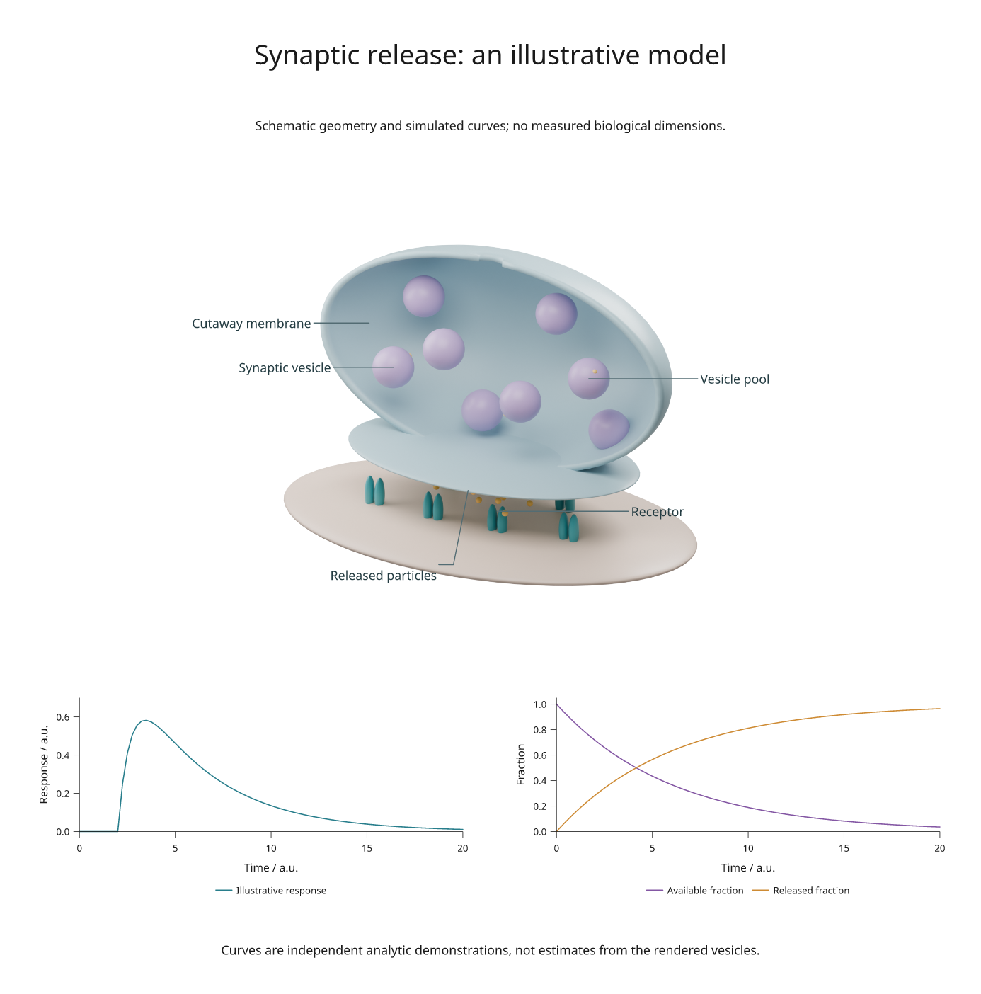
SVG · PDF · Figure recipe · Blender scene generator
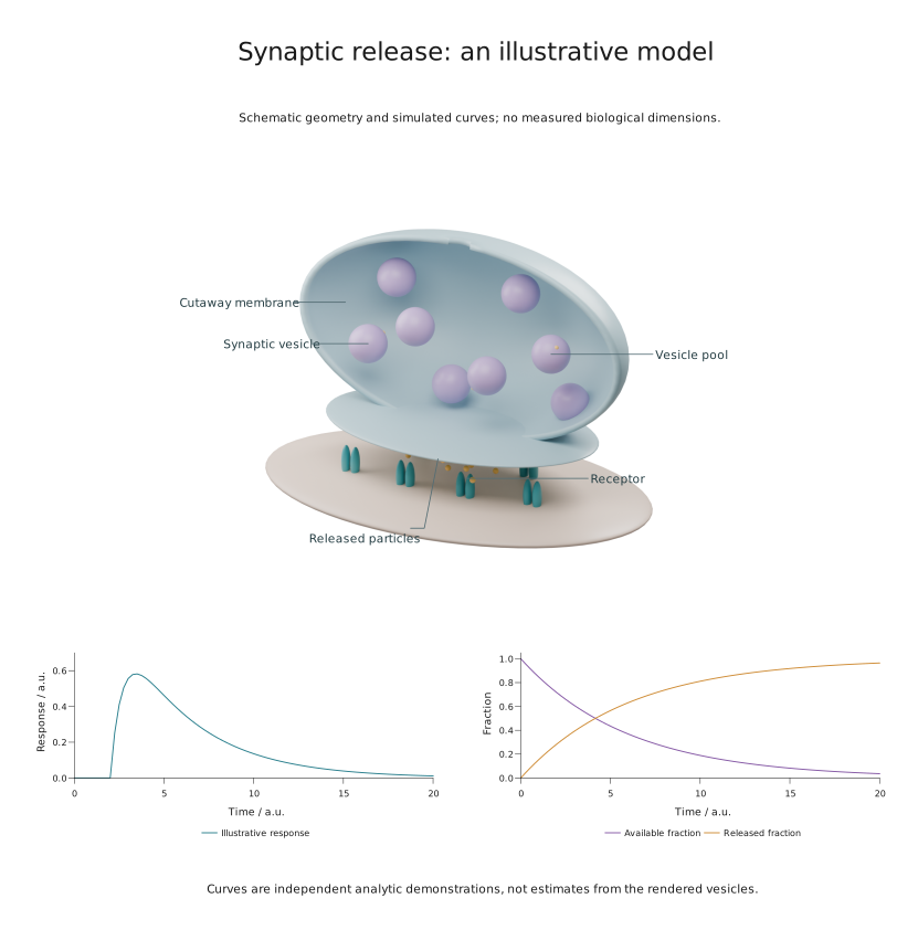
For a downloaded anatomical mesh, use the NIH model tutorial.
This is a schematic, with arbitrary geometry and simulated curves. Vesicle sizes, spacing and numbers do not represent measured anatomy. For calibrated microscopy and source segmentation meshes, see real organelle scenes.
Build the example
Use a checkout with Blender 4.5 LTS and Inklet's rendering extra installed. The example was rendered with Blender 4.5.13; no external meshes or textures are needed.
python -m pip install -e '.[render]'
python examples/scientific_blender.py --output out/scientific-blender
If Blender is outside PATH, add --blender /path/to/blender. The command
creates synapse.blend, SVG/PDF/PNG exports and review.txt. Cycles uses an
available GPU, with CPU fallback. The scene image is rendered at 300 DPI with
64 samples; see rendering setup for dependencies.
Open the .blend file to edit the materials, lights, camera or named structures.
The generator creates a half-shell membrane, an active zone, eight vesicles,
paired receptor shapes and release particles. The cutaway exposes otherwise
hidden objects; it is an explanatory construction, not a section measurement.
Add a label without rebuilding the scene
After running the example, this code renders or retrieves the cached camera view and places a label at a world coordinate:
import inklet as i

scene = i.render_blend('out/scientific-blender/synapse.blend',
    width=140, height=105, camera='Overview', engine='CYCLES',
    samples=64, dpi=300, passes=('depth',))
label = scene.annotate3d((-1.5, -.1, 1.8), 'Synaptic vesicle',
    side='w', clear=14, hidden='show', size=i.pt(8),
    leader_style={'stroke': '#536c73', 'stroke_width': .22})
art = i.overlay([scene.diagram, label], align='origin')
doc = i.document(width=220, margin=8)
doc.add('synapse', art)
doc.compile().save('labelled-synapse.svg', 'labelled-synapse.pdf')
The point is in Blender world coordinates; clear and stroke width are in
millimetres. size=i.pt(8) sets 8-point text. Keep align='origin': the label may
extend beyond the image without moving the camera projection.
This schematic uses hidden='show' to keep explanatory labels visible. For a
label that should disappear when its target is behind a surface, use
hidden='omit'; use hidden='dash' to indicate a hidden target. These options
require depth information. A screen-space label leader is not depth-tested.
See scene annotations for dimensions, arrows and angles.
Combine the scene with plots
The figure recipe places the scene across two columns, then assigns the two plots to explicit cells in the same row. Labels participate in measured layout; their extents are included when the scene is placed on the page.
The left curve uses (1 - exp(-(t-2)/0.8)) * exp(-(t-2)/4) after time 2 and zero
before it. The right curves use exp(-t/6) and its complement. Time and response
are arbitrary units. These formulas illustrate plot composition; they are not
fitted to the vesicles or a biological experiment.
Adapt it for scientific work
| Task | Change |
|---|---|
| Replace schematic geometry | Import your mesh into the .blend scene and retain a named camera |
| Label a biological structure | Choose a world point on its surface and check the rendered projection |
| Add a physical dimension | Supply an explicit world-to-physical scale to dimension3d() |
| Plot measurements | Replace the analytic curves with a typed CSV dataset |
| Review outputs | Inspect the figure at its intended print size and read the diagnostics |
For measured anatomy, retain source calibration and provenance through mesh import. Blender scene units alone do not establish a physical scale. The real microscopy example demonstrates this with organelle surfaces and associated measurements; the annotated laboratory shows a larger apparatus with detail views.