Slab projections and one shared region¶

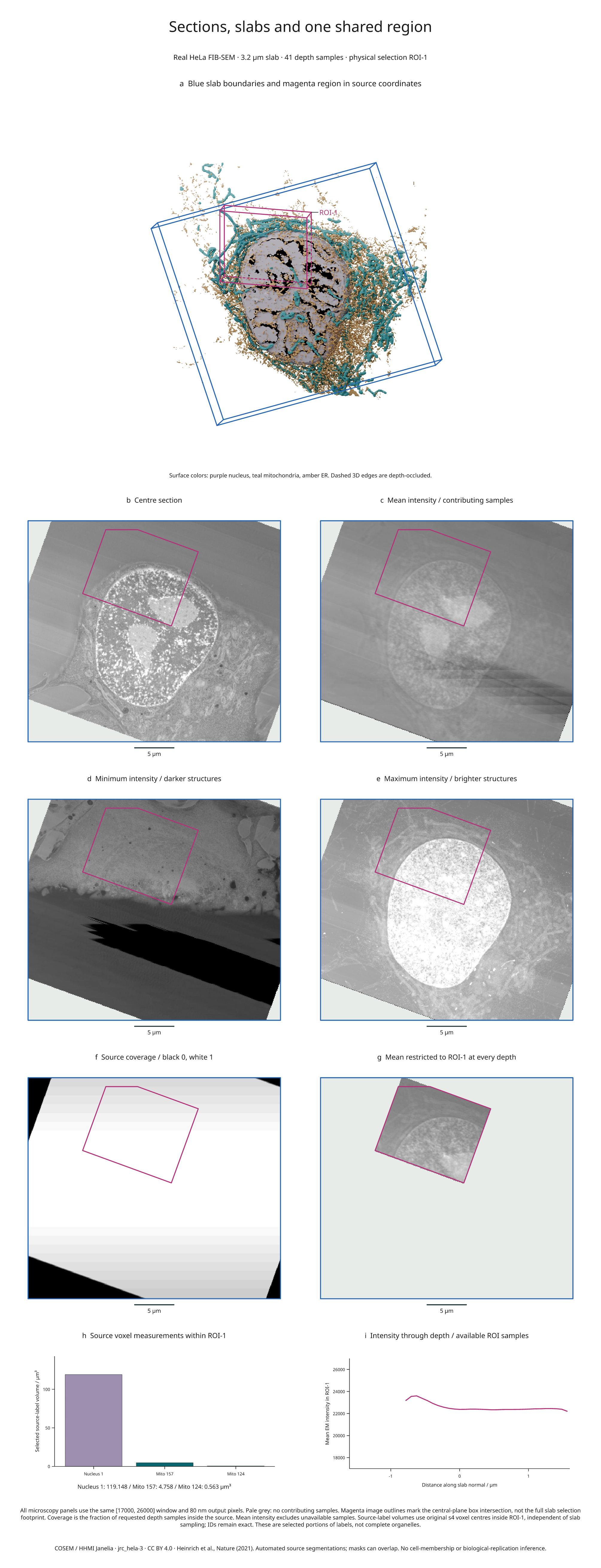
This nine-panel figure combines real HeLa electron microscopy, finite-thickness intensity projections, source coverage, a 3D organelle scene and measurements within a single physical region. The same ROI-1 box controls every selection; image resizing and projection sampling do not change the source-grid volumes.

Full-size figure · Executable recipe · Measurements and sampling evidence

Reproduce it¶

From 4.3 the example imports from inklet.volume; the inklet.experimental paths still work and, from 4.4, warn.

Use the v4.9.0 release checkout, the same locked COSEM source objects as the original real-biology example, and Blender 4.5 LTS:

git clone --branch v4.9.0 https://github.com/Mapika/inklet.git
cd inklet
python -m pip install -e '.[volume,render]'
python -m pip install -r examples/biology/requirements.txt
python examples/slab_biology.py --blender /path/to/blender

The recipe reuses verified data in out/real-biology/source.n5 and creates out/slab-biology/figure.svg, .pdf, .png, an HTML review, slabs.json and projection-arrays.npz. The NPZ contains unwindowed mean/min/max images, source contribution counts, the restricted mean and its contribution counts. Raw data and Blender scenes are generated locally and are not bundled. GPU rendering is preferred, with CPU fallback when no GPU is available.

Read the panels¶

• a: Blue edges bound a 3.2 µm slab around the oblique centre plane. Magenta edges show ROI-1, with world XYZ bounds (12, 0.4, 17) to (24, 2.8, 27) µm. Dashed edges are depth-occluded by scene geometry.
• b–e: The centre section and mean/minimum/maximum projections share the same 80 nm output pixels and [17000, 26000] display window. Each projection reduces 41 trilinearly sampled planes at equal-width bin midpoints. Minima emphasize darker EM structures; maxima emphasize brighter structures. Neither reconstructs a surface or represents a categorical label projection.
• f: Black is zero source coverage, white means all 41 requested midpoint samples contributed, and intermediate greys indicate partial coverage. This is sample coverage, not an uncertainty estimate or proof of continuous coverage.
• g: Mean intensity includes only samples inside both the source and ROI-1 at each depth. Pale grey indicates no contributors. The magenta image outline marks the box intersection with the centre plane; the selected slab footprint can extend beyond it.
• h: Volumes of source nucleus ID 1 and mitochondrial IDs 157 and 124 within the box use original s4 voxel centres and full voxel volumes. The measurement is independent of the slab's 41 samples and does not claim complete organelles.
• i: Each point is the mean over available ROI pixels at one slab depth. The evidence file includes its contributing pixel count. Missing depths break the line and are not plotted as zero intensity.

The slab and region API guide documents source-boundary handling, half-open region membership, projection normalization and measurement estimators. All projections exclude unavailable samples from the mean. Partial pixels keep full image opacity, which is why the coverage panel is separate.

Source and interpretation¶

This uses COSEM / HHMI Janelia, jrc_hela-3, with automated source segmentations at level s4. Its anisotropic source spacing remains 51.84 / 64 / 64 nm in ZYX. Output sampling does not improve acquisition resolution. Masks can overlap; these selected labels do not form a disjoint compartment partition. This is a visualization example, without cell-membership, biological-replication or uncertainty inference.

Data and derived figure: CC BY 4.0. Code: MIT. Source hashes and attribution are in the third-party notices and original example. Publication: Heinrich et al., Whole-cell organelle segmentation in volume electron microscopy, Nature 599, 141–146 (2021). This example adds finite slab projections, coverage maps, physical ROI selections and source-grid region measurements.