Slab projections and linked regions¶

Introduced in Inklet 3.1, Slab and BoxRegion are available from inklet.volume. Install inklet[volume] from PyPI as shown in the calibrated-volume guide. The inklet.experimental import paths used before 4.3 still work and return the same objects.

A slab samples a finite physical thickness around a Plane. A region is a box in world XYZ coordinates with an explicit selection ID. Use that same object for section outlines, projection restrictions, 3D edges and measurements on different calibrated sources.

A complete example¶

This small example uses simulated intensity and integer segmentation data.

import numpy as np
import inklet as i
from inklet.volume import Volume, Plane, Slab, BoxRegion

z, y, x = np.indices((13, 21, 25))
raw = Volume(x + 2*y + 3*z, (.5, .5, .5), 'um', source_id='simulated intensity')
labels = Volume(((x-12)**2 + (y-10)**2 + (z-6)**2 < 36).astype('uint16'),
                (.5, .5, .5), 'um', source_id='simulated labels')
plane = Plane((6, 5, 3), (1, 0, 0), (0, 1, 0), (21, 25), (.5, .5), 'um')
slab = Slab(plane, thickness=3, samples=12)
region = BoxRegion('ROI-1', (4, 3, 1), (8, 7, 5), 'um')

projection = raw.project_slab(slab, reduction='mean')
restricted = raw.project_slab(slab, reduction='mean', region=region)
measurement = region.measure(labels, label=1)
assert projection.counts.shape == plane.shape_yx
assert restricted.report()['selection']['selection_id'] == 'ROI-1'

image = projection.diagram(width=100, window=(0, 100))
outline = region.outline(plane, width=100, stroke='#b33279', stroke_width=.5)
linked = i.overlay([image, outline], align='origin')
doc = i.document(width=120, columns=1, margin=8)
doc.add('image', linked)
doc.add('scale', plane.scalebar(2, width=100))
figure = doc.compile()

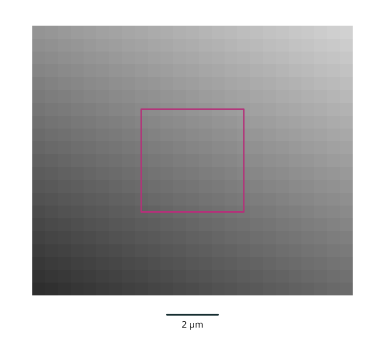
Rendered from the code above.

For a saved-camera render, draw each (start, end) in region.edges using rendered.path3d([start, end], hidden='dash', ...). All twelve edges use the original world coordinates. The real biology example includes this outline, projections, coverage and native-grid measurements in one figure.

Projection contracts¶

• thickness uses the plane's physical unit. samples is a positive integer. Samples lie at the midpoints of equal-width bins, from -thickness/2 + thickness/(2*samples) to +thickness/2 - thickness/(2*samples) along plane.normal_xyz. One sample is the centre section. Slab faces are geometric boundaries, not sampled endpoints.
• reduction='mean', 'max' or 'min' applies to intensity. Integer input is interpreted as intensity. Do not pass categorical label IDs: a maximum label ID or an averaged ID does not describe an organelle projection.
• Each sample uses trilinear interpolation and the same source-boundary rules as oblique sections. Outside-source samples are excluded. An optional region also excludes sample centres outside its box, at each depth.
• counts stores the contributing sample count per output pixel; coverage = counts / samples, and valid = counts > 0. All arrays are immutable. Coverage includes both source and region limits when selected. Mean divides by counts, never the requested count when samples are missing. Pixels with zero contributors store zero and render transparently.
• Partial pixels retain their computed intensity and full opacity. Display coverage separately when it affects interpretation. A fraction of 1 means every requested midpoint contributed; it is not a continuous coverage proof.
• Reduction streams one plane at a time with working memory proportional to output pixels, independently of sample count. The input volume still resides in memory. More output samples do not increase acquisition resolution.

Mean/max/min are established projection operations, also described in the ImageJ projection guide. Inklet records physical slab sampling, source identity and a contribution-count histogram in projection.report(). The arrays retain per-pixel evidence.

Region and measurement contracts¶

BoxRegion(selection_id, lower_xyz, upper_xyz, unit) requires finite, increasing bounds. Volume, plane and region units must match; there is no implicit unit conversion. A selection ID identifies the caller's chosen region, not a segmentation ID or an inferred biological object. Reusing it across panels does not require an interactive viewer.

region.mask(plane) selects output pixel centres with lower-inclusive, upper-exclusive membership. It does not include source coverage: combine it with section.valid when computing section statistics. region.intersection returns the plane/box boundary polygon clipped to the image extent, and region.outline draws it in image-centred page coordinates. Geometric outlines include boundary faces; membership at the upper face remains exclusive. For a slab, the central-plane outline is only that cross-section of the box, not the full projected selection footprint.

region.measure(volume, label=...) selects source voxel centres directly, retaining exact integer IDs including uint64. It returns selected label count and full-voxel volume, alongside the available source voxel count and grid volume within the region. Background ID 0 is allowed; absent IDs return zero. Values outside the source are unavailable, not background. The result depends on the supplied source grid and includes full voxel volumes at selected centres; it does not calculate partial-voxel intersections. It is independent of slab sampling, image width and output resolution. It does not infer object completeness, cell membership or uncertainty.