Uncertainty and supplied intervals¶

Inklet draws the bounds or error magnitudes you supply; it does not infer a confidence interval from raw observations. State what the interval means and how another calculation produced it. Distinguish absolute bounds from distances around a central estimate.

All values below are illustrative. Each snippet can be run independently with core Inklet; PNG preview generation additionally uses the render extra. Run a block as a script from the repository root, or paste it into a Python session. Every block creates its own document and writes SVG and PDF.

Bands¶

A band joins supplied lower and upper bounds over x. Both arrays contain absolute y coordinates. Draw the central line afterward.

import inklet as i
x = list(range(13))
mean = [2.0, 2.25, 2.55, 2.7, 2.95, 3.15, 3.35, 3.6, 3.72, 3.95, 4.1, 4.28, 4.5]
low = [1.45, 1.72, 2.05, 2.1, 2.42, 2.55, 2.72, 3.05, 3.0, 3.35, 3.4, 3.68, 3.82]
high = [2.55, 2.82, 3.0, 3.35, 3.5, 3.8, 3.98, 4.15, 4.52, 4.55, 4.82, 4.88, 5.18]
p = i.plot_spec(x=(0, 12), y=(0, 5.6), height=44)
p.band(x, low, high, fill='#b8d6cd', stroke='none')
p.line(list(zip(x, mean)), stroke='#288675', stroke_width=.5)
p.grid(x=False, y=True, count=5, stroke='#e1e7e4', stroke_width=.15)
p.axes(x='Time / s', y='Estimate / a.u.')
doc = i.document(width=110)
doc.add('band', p)
doc.save('band.svg', 'band.pdf')

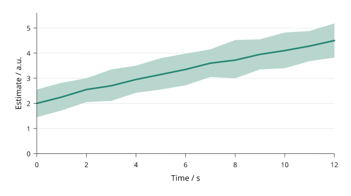
Rendered from the code above. The 13-point centre line and changing bounds are supplied illustrative values; the band is not a confidence interval.

Error bars¶

Error bars show distances from each estimate. yerr and xerr accept symmetric magnitudes or one (down, up) pair per point. Convert absolute interval limits by subtracting the central estimate. cap is the half-width of an end cap in millimetres.

import inklet as i
points = [(1, 2.1), (2, 3.35), (3, 2.85), (4, 4.15), (5, 3.75)]
p = i.plot_spec(x=(0, 6), y=(0, 5.5), height=44)
p.errorbars(points, yerr=[(.25, .4), (.45, .3), (.35, .55), (.5, .38), (.28, .46)],
            xerr=[.08, .12, .1, .14, .09], cap=1, stroke='#24698c')
p.scatter(points, size=1.8, color='#24698c')
p.grid(x=False, y=True, count=5, stroke='#e1e7e4', stroke_width=.15)
p.axes(x='Dose / µM', y='Response / mV')
doc = i.document(width=110)
doc.add('errorbars', p)
doc.save('errorbars.svg', 'errorbars.pdf')

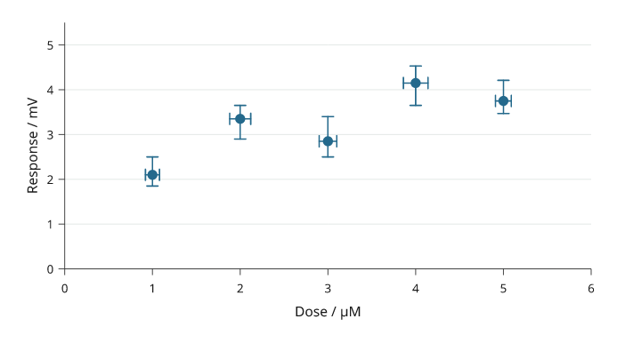
Rendered from the code above. Five illustrative dose–response estimates have asymmetric response distances and supplied dose uncertainty.

Whiskers that reach zero on a log axis. A log axis cannot place a bound of zero or below, and a fitted estimate often has one. Such a whisker runs to the bottom of the axis and ends in an open arrowhead, which shows that it continues past the axis, and the log scale is kept. floor="none" leaves the arrowhead off. The point itself must still be above zero. symlog() changes the whole axis instead, so use it only when the axis has to reach zero.

import inklet as i
p = i.plot_spec(x=(0.05, 300), y=i.log((1e-4, 1)), height=44)
p.errorbars([(0.6, 8e-4), (30, 3e-3)], yerr=[(8e-4, 6e-3), (1e-3, 1e-3)], cap=.7)
p.axes(x='Dose / µM', y='Coupling')
doc = i.document(width=110)
doc.add('floor', p)
doc.save('floor.svg', 'floor.pdf')

Line with errors¶

A line can show supplied uncertainty as a band or error bars. err uses error magnitudes, like errorbars; err_style="band" shades the spread and err_style="bars" draws whiskers. The uncertainty is drawn before the line.

import inklet as i
p = i.plot_spec(x=(0, 12), y=(0, 6), height=44)
p.line([(0, 1.5), (1, 1.95), (2, 2.35), (3, 2.85), (4, 3.1),
       (5, 3.55), (6, 3.85), (7, 4.05), (8, 4.35), (9, 4.55),
       (10, 4.78), (11, 5.0), (12, 5.18)],
       err=[.28, .34, .3, .42, .38, .45, .36, .5, .44, .52, .46, .58, .5],
       err_style='band', stroke='#b86443', name='Supplied estimate')
p.grid(x=False, y=True, count=5, stroke='#e1e7e4', stroke_width=.15)
p.axes(x='Time / s', y='Estimate / a.u.').legend(side='bottom')
doc = i.document(width=110)
doc.add('line-errors', p)
doc.save('line-errors.svg', 'line-errors.pdf')

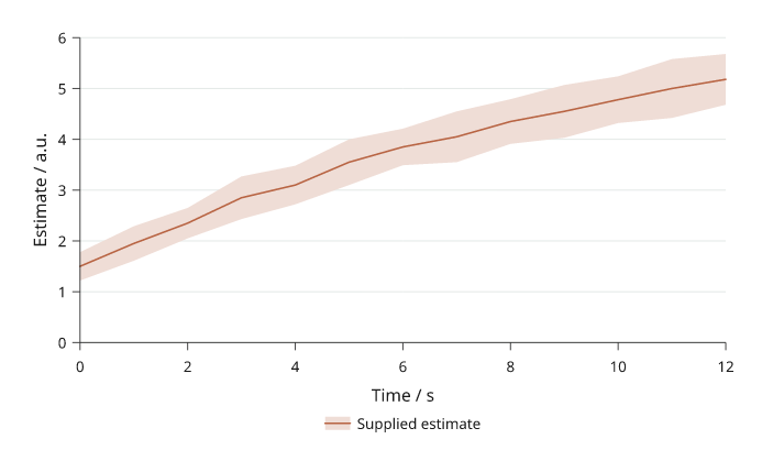
Rendered from the code above.

Reusable series¶

A Series keeps the name, values, colour and absolute bounds together. Use plot_spec().series() when several panels should share that definition. The lower and upper arrays are absolute bounds, not error magnitudes.

import inklet as i
times = list(range(7))
control = i.Series('Control', times, [1.3, 1.65, 1.95, 2.2, 2.5, 2.72, 2.95], '#24698c',
                   [1.0, 1.32, 1.6, 1.82, 2.08, 2.3, 2.5],
                   [1.6, 1.98, 2.3, 2.58, 2.9, 3.12, 3.4])
treatment = i.Series('Treatment', times, [1.5, 1.95, 2.3, 2.72, 3.0, 3.32, 3.6], '#288675',
                     [1.15, 1.58, 1.9, 2.3, 2.55, 2.85, 3.08],
                     [1.88, 2.3, 2.7, 3.1, 3.45, 3.78, 4.12])
p = i.plot_spec(x=(0, 6), y=(0, 4.5), height=44)
p.series(control, stroke_width=.45)
p.series(treatment, stroke_width=.45)
for series in (control, treatment):
    p.series(series, uncertainty=False, stroke_width=.45)
p.grid(x=False, y=True, count=5, stroke='#e1e7e4', stroke_width=.15)
p.axes(x='Time / s', y='Estimate / a.u.').legend(side='bottom')
doc = i.document(width=110)
doc.add('series', p)
doc.save('series.svg', 'series.pdf')

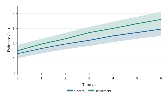
Rendered from the code above. The reusable definitions compare illustrative Control and Treatment trajectories with absolute, nonconstant bounds; these bands do not claim confidence intervals.

The final line-only pass keeps both trajectories visible above the overlapping bands. Reusing a series name keeps one combined entry in the legend.

Forest plots¶

i.forest draws one row per study or subgroup: a square at the point estimate on a line across its confidence interval, a diamond for a summary row and a bold label for a group header. Rows are listed top to bottom as mappings with label, estimate, low, high and optionally weight, summary=True or header=True; a bare string is a header, and a tuple (label, estimate, low, high) is a study. Rows after a header are indented until the next summary. With weights, the square areas follow the weights.

log=True puts x on a log axis, for odds or hazard ratios, and draws the line of no effect at 1; on a linear axis it is at 0. limits= fixes the x range, and an interval that runs past it ends in an arrowhead at the limit. left= and right= list the text columns on each side: 'label', 'ci' (the estimate and interval as text, with digits decimals: 0.72 (0.55–0.94), or −0.02 (−0.03 to −0.01) with minus signs and "to" when a bound is negative), 'estimate', 'weight', any other key of the row mappings, or a (header, key or function) pair. Numbers are right-aligned. measure names the estimate in the column headers. inklet.plot.forest_layout returns the parsed rows, limits and clipped interval ends without drawing. text_size= sets the columns' type size and gap= the space between them.

i.quick.forest fits its cell: the plot narrows to 20 mm, the gaps between columns close, then a right-hand 'ci' or 'estimate' column is dropped with a warning (the plot still draws every estimate and interval), and then the columns' type is set smaller, down to the preset's minimum text size. A forest that is still too wide raises a LayoutError listing these steps.

import inklet as i

rows = [
    'Adults',
    {'label': 'Ahmed 2019', 'estimate': .72, 'low': .55, 'high': .94, 'weight': 18.2, 'n': 812},
    {'label': 'Berg 2020', 'estimate': .91, 'low': .62, 'high': 1.33, 'weight': 9.4, 'n': 355},
    {'label': 'Chen 2021', 'estimate': .64, 'low': .38, 'high': 1.08, 'weight': 6.1, 'n': 210},
    {'label': 'Subtotal', 'estimate': .76, 'low': .63, 'high': .92, 'summary': True},
    'Children',
    {'label': 'Diaz 2018', 'estimate': 1.12, 'low': .70, 'high': 1.80, 'weight': 6.3, 'n': 240},
    {'label': 'Evans 2022', 'estimate': .58, 'low': .12, 'high': 6.4, 'weight': 1.0, 'n': 31},
    {'label': 'Subtotal', 'estimate': 1.02, 'low': .66, 'high': 1.58, 'summary': True},
    {'label': 'Overall', 'estimate': .81, 'low': .69, 'high': .95, 'summary': True},
]
plot = i.forest(rows, log=True, limits=(.2, 5), measure='OR', right=['ci', 'n'],
                label='Odds ratio', width=34)
doc = i.document(width=120)
doc.add('forest', plot)
doc.save('forest.svg', 'forest.pdf')

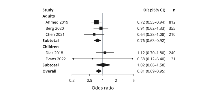
Illustrative numbers. The Evans 2022 interval runs past both axis limits and ends in arrowheads; its square is the smallest because its weight is.

Next steps¶

Compare plot types, configure axes and scales, or arrange several panels. For exact options, see the API.